Introduction
AI inference is expensive in various ways
I first started using SGLang and other inference engines, such as vLLM, to explore potential energy optimisation opportunities for distributed inference. In past years, most software developers have been enjoying the perks of energy consumption reduction thanks to the advancement in hardware: various finFET versions to GAA to reduce the static energy loss, NVLink replacing PCIe to speed up the memory movement, lowering of the circuit voltage and thus reduce dynamic energy loss, etc. All of these hardware improvements have led to an almost free energy reduction from the software developer’s perspective.
We, of course, can wait for the next generation of hardware, perhaps a wafer-scale engine, 3D chiplet stacking, or even optical computing to let us once again enjoy the free perks of energy consumption reduction. But each generation of our state-of-the-art hardware: CPU + GPU (or other accelerators) lasts about 3-5 years per data centre cycle. And electricity costs are only going up, accounting for almost 50% of the total monthly cost, after amortising the hardware cost. Hence, there is still a need to optimise energy consumption at the software and system levels.
Some thoughts on reducing energy consumption
Initially, my two main ideas for distributed inference are quite simple: (1) Don’t deploy more model instances than necessary. This enables us to reduce dynamic energy loss in idle model instances. (2) If we need to deploy more model instances, we should at least make sure that the model instances are configured in their best parameters, perhaps the lowest energy consumption given Service-Level Objectives and cost constraints. I did some preliminary exploration of these two ideas and found that we could potentially use Multi-Objective Bayesian Optimisation (MOBO) to find Pareto frontier configurations. On top of that, given the Pareto configurations from MOBO, we could then use Mixed Integer Linear Programming as a “scheduler” to scale the number of model instances needed and how to route each request to the model instances, sort of like the Job Service Placement and Request Routing problem from the Mobile Edge Computing literature. After a while, I realised that I was basically auto-tuning the system configurations and trying to reduce energy consumption by matching the parallelism strategies to the hardware configuration, sort of treating it like a black box.
Exploring GPU kernel-level optimizations
However, I don’t wanna just stop at the outer layer scheduling part without knowing what are the fundamentals calculations that the GPU is performing, that is when i have decided that I want to at least explore how inference engine like SGLang is creating customize kernels for each type of model so that they can optimize their performance, and potentially lower the energy consumption when the efficiency of algorithm and kernel is improving.
A general view
As I plan to investigate into kernel level, let’s start with how Python and C++ can co-exist in one repository: where we can write kernel in C++ and expose it to Python, why why we are doing this. To investigate into how customize kernels are being used in LLM inference engine, we should learn the basic concepts of Python/C++ bindings, and the ML compiler stack.
Python/C++ Bindings
Some basics about Python/C++ Bindings
In the ML and AI field, Python is basically the most used language. This is because it is beginner friendly and it has a very rich ecosystem of libraries. However, Python as an interpreted language means that it is not the fastest language in the world because it is not compiled to machine code before it is run. In order to speed up Python, people have been using Just-in-Time (JIT) compilers, such as Numba, to compile Python code to machine code at runtime. In addition to these, there are also libraries written in C++ but with Python user-friendly API, such as NumPy, which code is compiled to machine code at compile time, making the “python code” much faster.
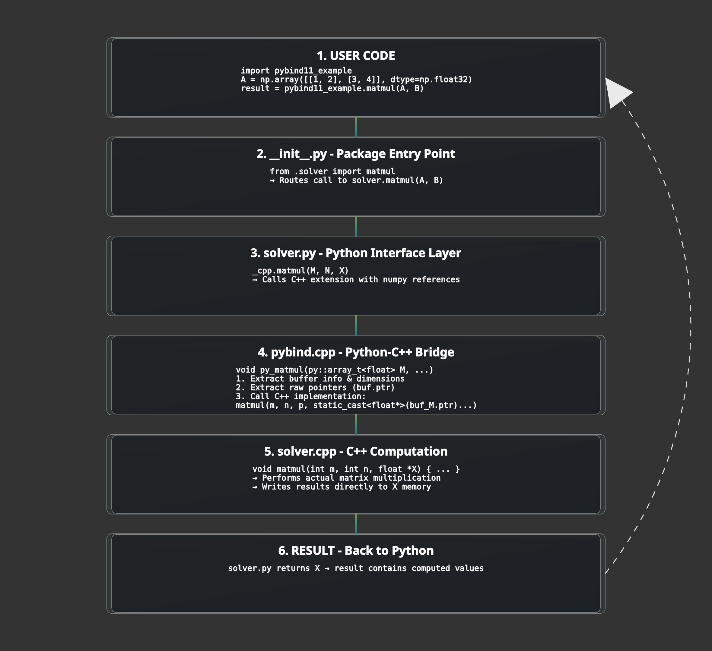
To combine the usage of both Python and C++, we can use pybind11. For example, let’s take matrix-matrix multiplication (inspired by https://github.com/xflash96/pybind11_package_example/tree/main). We can write a C++ code to perform matrix-matrix multiplication and then use pybind11 to wrap it in a Python function. This allows us to use the speed of C++ while maintaining the ease of use of Python.
Code Structure:
example
├── pybind11_example      # The Python package
│   ├── __init__.py	      #    API definitions
│   └── solver.py         #    Python implementation
├── src				      # The C++ extension
|   ├── solvers.cpp 	  #    C++ implementation
|   ├── solvers.h		  #    C++ header
|   └── pybind.cpp		  #    Bindings to Python
└── setup.py
We will start with init.py: the entry point of the package, defining which function can be called by the users
This is where the init.py point to –> solver.py: contains the function in the package, contains the algorithm and maybe calling the C++ extension
Under another src/ folder, we have solver.cpp: the algorithm in cpp, will be compiled to shared library while building the python package
Under the same folder, solver.h: defining the function signature
pybind.cpp: explaining the binding, here we use the raw point to achieve zero copy, aka the cpp code will be performing in memory operations.
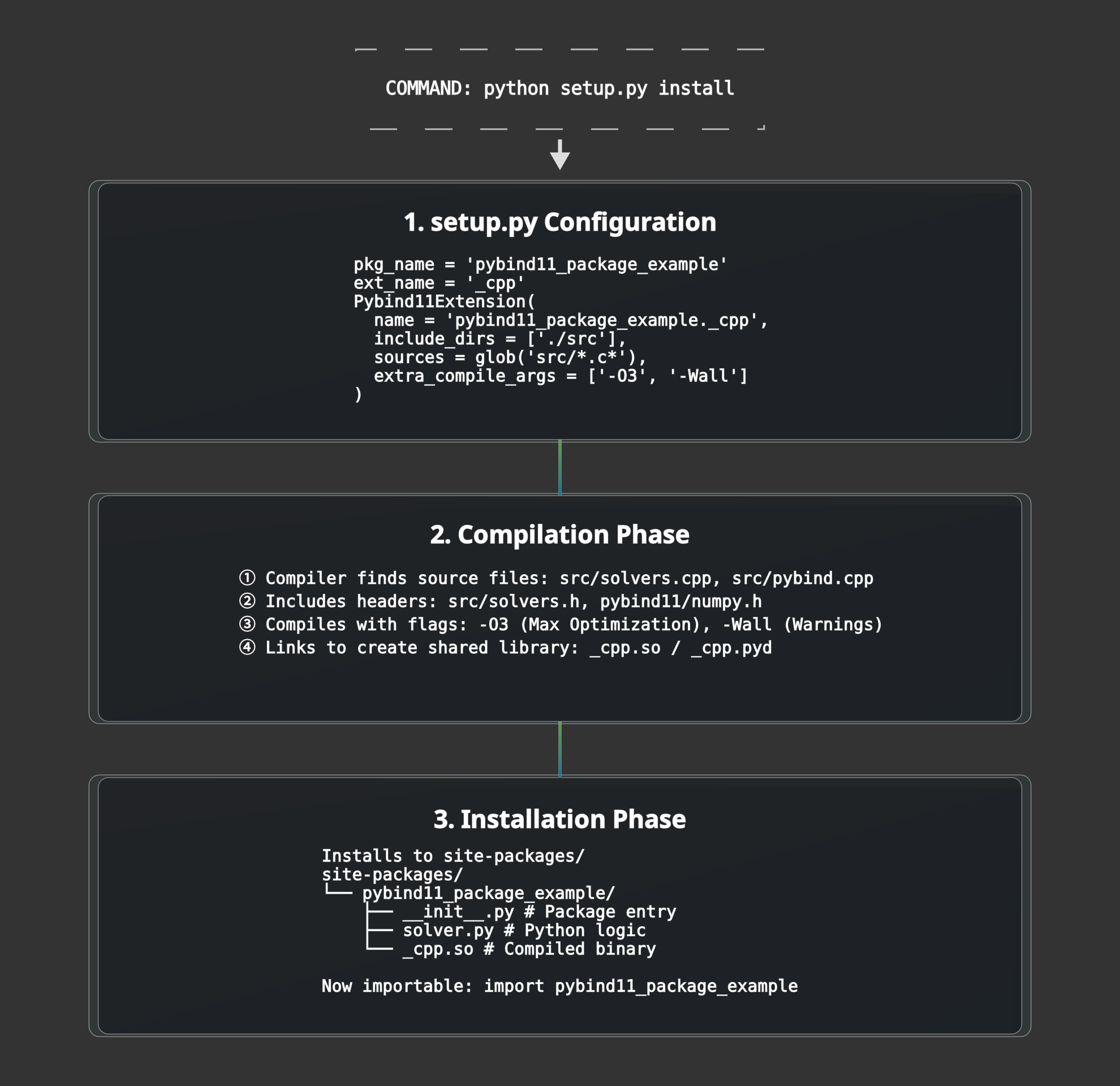
For the package, we have setup.py: defining how to build the package
Overall, the execution flow is as follows:
Overall Build Process (One-time):
From these, user can accelerate their matrix multiplication function by just calling import pybind11_example; pybind11_example.matmul(M, N), pretty cool!
Feel free to skip if you are already familiar with it :)
ML Compiler Framework
Inspirations from LLVM
In the ML space, the compiler itself is heavily inspired by LLVM. In LLVM, there are 3 main components: the front-end framework (Clang, C++, etc.), the optimiser, and the back-end framework (CPU, GPU, NPU, etc.). In LLVM, the front-end framework converts the source code to LLVM IR (Intermediate Representation), the optimiser optimises the LLVM IR, and the back-end framework converts the optimised LLVM IR to machine code for the target hardware.
Flexibilities of MLIR
In ML, the compiler uses multi-level IRs. The front-end framework will convert the source code to MLIR (Machine Learning Intermediate Representation), the optimiser will optimise the MLIR, and the back-end framework will convert the optimised MLIR to machine code for the target hardware. The world of ML is quite messy, before the use of MLIR, there were many different frameworks and libraries, each with its own IR and optimisation passes. This makes it difficult to share code and optimisations between frameworks. MLIR was created to solve this problem by providing a common IR and optimisation framework for ML. It allows developers to define multiple dialects, e.g., a Linalg dialect, a Vector dialect, and a GPU dialect, which can coexist and interoperate.
MLIR has several benefits. First of all, it is easier to port the code to different hardware. When MLIR becomes generalizable, it also means it may have traded a bit of performance. This is because the general MLIR compiler is not tailored to any specific hardware, so it cannot fully utilise the hardware’s potential. To solve this issue, developers often had to code in CUDA C++ for a single thread and carefully calculate where that thread sits in a block in hardware to fully extract the performance. This is very time-consuming and error-prone. To solve this issue, Triton is written to combine the best of both worlds, it uses a Python-based front-end that lowers into specialised MLIR dialects. Unlike a ‘general’ MLIR compiler, Triton’s MLIR passes are opinionated: they specifically automate the ‘hard’ parts of GPU programming, like memory coalescing and software pipelining, that developers previously had to do manually in CUDA C++. Finally, it uses a back-end (often LLVM) to convert the optimised MLIR representation into hardware-specific machine code.
Hardware advances outpace compiler’s ability to keep up
However, hardware advances often outpace the compiler’s ability to keep up, so the compiler needs to be updated to support new hardware features. For example, NVIDIA’s Blackwell Architecture introduces new hardware features, such as the Tensor Core 5 with native FP4 support, which are not fully supported by the current MLIR compiler. To support these new features, the MLIR compiler needs to be updated to include new optimisation passes and code generation strategies. This is a time-consuming and error-prone process, and it is one of the main challenges in developing ML compilers. Hence, developers still need to write high-performance kernels in CUDA C++ to squeeze out the last few percentage points of performance on the new hardware. And I think this is why SGLang started developing its own SGL-Kernel, targeting the Blackwell architecture, with advanced algorithms such as MoE blockwise matrix multiplication.
Digging… ⛏️the rabbit hole in SGLang
To understand the computational bottleneck of MoE models on SGLang, we need to understand how SGLang design their server architecture before they dispatch the code on GPU. In MoE architecture, the most time consuming operation is the matrix multiplication between the input tokens and the weights of the model. Notably, it is called MoE Blockwise Scaled Matrix Multiplication. Before we optimize the code, we first have to understand how the code is being used. In the following section, we will trace the operation in SGLang server, understanding how their command line interface will ultimately dispatch the MoE code on GPU.
Starting Point: The Command Line Interface
We will start from the Python API for SGLang. For a user to run a model instance for online serving, they can use python -m sglang.launch_server --model-path <model_path> --other-args. The launch_server function will then call sglang.server.run_server to start the server.
Server Initialization & Process Management
In the SGLang repository, the entry point of the server is python/sglang/launch_server.py. If the default arguments are used, it will call python/sglang/srt/entrypoints/http_server.py which allows Inter Process Communication and then calls launch_server to start the server through subprocesses _launch_subprocesses(). The _launch_subprocesses() function is from python/sglang/srt/entrypoints/engine.py. The engine file runs tokenizer, detokenizer and scheduler subprocesses. Under the engine.py file, it also calls run_scheduler_process() from python/sglang/srt/managers/scheduler.py to start the scheduler process. The scheduler process is the core of SGLang, it is responsible for different parallelisation strategies in the execution of the model, such as tensor parallelism, pipeline parallelism, and data parallelism.
Model Loading Phase
During scheduler initialization, Scheduler.__init__() triggers the model worker setup. This creates a TpModelWorker instance, which in turn initializes a ModelRunner, then calls initialize() followed by load_model() to begin the actual model loading process. The model loading begins with get_model_loader() from python/sglang/srt/model_loader/loader.py, which returns a DefaultModelLoader instance based on the configuration. The loader performs the critical step of instantiating the model class via model_class(**kwargs). This dynamically calls the appropriate model constructor based on the model architecture (e.g., DeepSeek V2, Mixtral, Qwen2-MoE) from files like python/sglang/srt/models/deepseek_v2.py or python/sglang/srt/models/mixtral.py.
DeepSeek V2 Model Instantiation
Using DeepSeek V2 as an example, the instantiation chain flows through DeepseekV2ForCausalLM.__init__() → DeepseekV2Model.__init__() → DeepseekV2DecoderLayer.__init__(). At each decoder layer, DeepseekV2MoE.__init__() is called. This MoE layer constructor calls get_moe_impl_class() from python/sglang/srt/layers/moe/ep_moe/layer.py to select the appropriate MoE implementation based on quantization settings and backend configuration. For DeepSeek models with expert parallelism, this returns DeepEPMoE, which is immediately instantiated. The DeepEPMoE.__init__() creates the MoE engine, allocating memory for expert weights and setting up the routing mechanism. After all layers are initialized, weights are loaded from disk and copied into the allocated parameters. At this point, the model is fully loaded in GPU memory and ready for inference.
Runtime: Inference Forward Pass
When an inference request arrives, it flows through the scheduler into DeepseekV2MoE.forward(), which handles the runtime computation. The forward pass delegates to DeepEPMoE.forward() from python/sglang/srt/layers/moe/ep_moe/layer.py, which orchestrates the three main MoE operations: routing, expert computation, and output combining. The run_moe_core() method performs the actual expert computation. For W4AFP8 quantized models, it calls W4AFp8MoEMethod.apply_deepep_normal() from python/sglang/srt/layers/quantization/w4afp8.py, which handles the quantization-aware computation. This method invokes cutlass_w4a8_moe_mm() in the Python layer from python/sglang/srt/layers/moe/cutlass_w4a8_moe.py, which wraps the low-level kernel call.
The Python-to-CUDA Bindings
The Python wrapper in sgl_kernel/moe.py uses PyTorch’s operator registration system via torch.ops.sgl_kernel::cutlass_w4a8_moe_mm to dispatch to the C++ implementation. The C++ extension registered in sgl-kernel/csrc/common_extension.cc using TORCH_LIBRARY_FRAGMENT binds the Python call to the actual kernel implementation. The CUDA kernel implementation in sgl-kernel/csrc/moe/w4a8_moe_kernel.cu prepares the computation by calling w4a8_grouped_mm_c3x(), which launches the optimized kernel. This function instantiates CUTLASS templates (cutlass::gemm::kernel::GemmUniversal) with the specific data types and tile sizes for the operation. Finally, the templated CUTLASS kernel compiles down to the actual GPU kernel __global__ void fused_moe_kernel<<<>>>(), which executes on the GPU hardware. This kernel performs the highly optimized matrix multiplications for all selected experts in parallel, leveraging GPU tensor cores and shared memory for maximum throughput. The computed results flow back through the call stack, are combined with the routing weights, and return as the final MoE layer output, continuing through the remaining transformer layers until the model produces its prediction.
The full execution flow can be visualize as:
Click here to expand the full view.
python -m sglang.launch_server
    ↓
sglang/launch_server.py
    ↓
sglang/srt/entrypoints/http_server.py::launch_server()
    ↓
sglang/srt/entrypoints/engine.py::_launch_subprocesses()
    ↓
sglang/srt/entrypoints/engine.py::_launch_scheduler_processes()
    ↓
sglang/srt/managers/scheduler.py::run_scheduler_process()
    ↓
sglang/srt/managers/scheduler.py::Scheduler.__init__()
    ↓
sglang/srt/managers/tp_worker.py::TpModelWorker.__init__()
    ↓
sglang/srt/model_executor/model_runner.py::ModelRunner.__init__()
    ↓
sglang/srt/model_executor/model_runner.py::ModelRunner.initialize()
    ↓
sglang/srt/model_executor/model_runner.py::ModelRunner.load_model()
    ↓
sglang/srt/model_loader/loader.py::get_model_loader()
    ↓
sglang/srt/model_loader/loader.py::DefaultModelLoader.load_model()
    ↓
sglang/srt/model_loader/loader.py::_initialize_model()
    ↓
sglang/srt/model_loader/loader.py::model_class(**kwargs)
    ↓
sglang/srt/models/deepseek_v2.py::DeepseekV2ForCausalLM.__init__()
    ↓
sglang/srt/models/deepseek_v2.py::DeepseekV2Model.__init__()
    ↓
sglang/srt/models/deepseek_v2.py::DeepseekV2DecoderLayer.__init__()
    ↓
sglang/srt/models/deepseek_v2.py::DeepseekV2MoE.__init__()
    ↓
sglang/srt/layers/moe/ep_moe/layer.py::get_moe_impl_class()
    ↓
sglang/srt/layers/moe/ep_moe/layer.py::DeepEPMoE.__init__()  # MoE engine started
    ↓
    ↓ [Model loaded, ready for inference]
    ↓
━━━━━━━━━━━━━━━━━━━━━━━━━━━━━━━━━━━━━━━━━━━━━━━━━━━━━━━━━━━━━━━━━━━━━━
    ↓ [RUNTIME: Forward pass]
    ↓
sglang/srt/models/deepseek_v2.py::DeepseekV2MoE.forward()
    ↓
sglang/srt/layers/moe/ep_moe/layer.py::DeepEPMoE.forward()
    ↓
sglang/srt/layers/moe/ep_moe/layer.py::DeepEPMoE.run_moe_core()
    ↓
sglang/srt/layers/quantization/w4afp8.py::W4AFp8MoEMethod.apply_deepep_normal()
    ↓
sglang/srt/layers/moe/cutlass_w4a8_moe.py::cutlass_w4a8_moe_mm()
    ↓
sgl_kernel/moe.py::cutlass_w4a8_moe_mm()
    ↓
torch.ops.sgl_kernel::cutlass_w4a8_moe_mm
    ↓
sgl-kernel/csrc/common_extension.cc::TORCH_LIBRARY_FRAGMENT
    ↓
sgl-kernel/csrc/moe/w4a8_moe_kernel.cu::w4a8_grouped_mm_c3x()
    ↓
cutlass::gemm::kernel::GemmUniversal<...>
    ↓
__global__ void fused_moe_kernel<<<>>>()  # GPU kernel execution
Digging… ⛏️ another rabbit hole in SGLang-Kernel
Now, imagine we have the latest Blackwell Architecture in our hand, but Triton is not ready to fully exploit its latest hardware features, such as FP4 and the Tensor Memory Accelerator. This is where NVIDIA’s Cutlass comes into play for optimisation. The benefits of writing a custom cutlass kernel for the latest architecture are also recognised by the SGLang developers, which is why, under SGLang-Kernel, we can see a cutlass implementation of various GEMM kernels specifically targeting the Blackwell architecture. An example can be shown at: sgl-kernel/csrc/csrc/moe/fp8_blockwise_moe_kernel.cu.
While I was looking at specific kernel for MoE (mainly because MoE only activating subset of parameters during inference, maintaining its model capability while reducing the need for extra computation, thus reducing energy), I found that currently there’s cutlass implementation of MoE blockwise matrix multiplication for NVFP4 but not for FP8, hence when a user with Blackwell architecture is calling a kernel in FP8, the suboptimal Triton kernel that’s tailored for previous generations of hardware architecture is used. Realising this, I wanted to try implementing the cutlass kernel in FP8, for educational purposes and exploration.
The Math in the MoE Kernel: Scaled Matmul with Quantization
The Core Problem
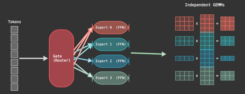
Under the MoE MLP layer, each expert is essentially an FFN. Each layer also consists of a gating mechanism decides which expert to route each token through. This also means that for each layer, we have to compute several independent matrix multiplications, one for each expert, and potentially with a different number of rows because the number of tokens routed to each expert varies. A well-optimised kernel would have fused all computations into a single kernel to avoid the overhead of launching multiple kernels. This is the grouped GEMM problem.
Quantization and Scaled Matmul
To reduce memory bandwidth requirements, we quantise the weight matrix from FP16 to FP8 and to INT4. However, to maintain the model’s capability, developers usually dequantize the matrix before performing the matrix multiplication, thereby using higher precision and wider ranges for calculation.
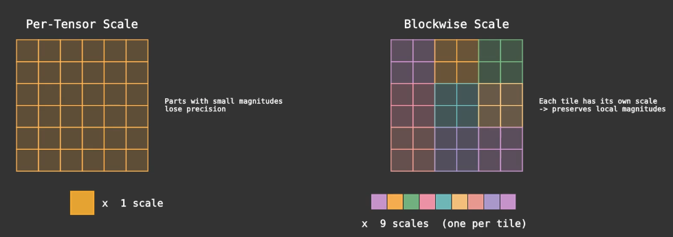
Originally, developers used tensor-wise scaling by assigning one scaling factor to each tensor. However, this is not optimal because different parts of the tensor may differ widely in magnitude, leading to suboptimal quantisation. Hence, blockwise scaling is a better choice, where we assign a single scaling factor to each tensor block, allowing each tensor to have different scaling factors within itself. This maintains the inference accuracy while reducing the memory bandwidth requirement.
To summarise, direct matrix multiplication with lower-precision parameters is not optimal because it loses accuracy. We dequantize the matrix using our scaling factors (essentially a linear mapping from lower to higher precision) before performing the matrix multiplication. This is the “scaled matmul” approach. The benefit is that we can use lower-precision parameters to store the matrix, reducing memory bandwidth requirements while maintaining inference accuracy at high precision.
Kernel - Cutlass Solution
To write the FP8 blockwise kernel, we use the cutlass template provided by NVIDIA. CUTLASS is a collection of abstractions for implementing high-performance matrix-matrix multiplication (GEMM) and related computations at all levels and scales within CUDA. We can then use the template to generate the kernel for different hardware architecture.
The kernel is focused on the grouped GEMM problem, in FP8 on 5060Ti, and structured in 2 layers: Dispatch and Kernel. Dispatch is responsible for dispatching the kernel to the GPU, while Kernel is responsible for the actual computation. For each GEMM, they each have their own (M,N,K) dimension where A is size (M,K), B is size (K,N) and C the output is size of (M,N) in A x B = C.
Diving into the Dispatch code, this is where developers define the problem size, tensor shape, precision and scheduling method for matmul / epilogue stages. Developers can decide the kernel configurations based on the matmul (M,N,K) shape. In this case, we use the cutlass template to generate the kernel for different hardware architecture. For matmul with very large M and K dimention, for example, batched requests for high hidden dimensions, it means that we have to perform many dot products in iterations. With a higher M, a kernel has more output tiles, this gives the scheduler more independent tasks to dispatch across SMs, leading to higher SM occupancy. With a higher K, a kernel need to do more dot products to accumulate the result in one iteration, leading to higher usage of Shared Memory. One interesting trick is when we have a smaller M, we could use matrix transposition trick where (C^T = B^T x A^T), thus shifting the M to be the K in the matmul, leading to higher SM occupancy during the calculation.
Dispatch Cutlass Code
template <typename OutType>
void sm120_fp8_blockwise_group_mm_dispatch_shape(
    torch::Tensor& output,
    torch::Tensor& a_ptrs,
    torch::Tensor& b_ptrs,
    torch::Tensor& out_ptrs,
    torch::Tensor& a_scales_ptrs,
    torch::Tensor& b_scales_ptrs,
    const torch::Tensor& a,
    const torch::Tensor& b,
    const torch::Tensor& scales_a,
    const torch::Tensor& scales_b,
    const torch::Tensor& stride_a,
    const torch::Tensor& stride_b,
    const torch::Tensor& stride_c,
    const torch::Tensor& layout_sfa,
    const torch::Tensor& layout_sfb,
    const torch::Tensor& problem_sizes,
    const torch::Tensor& expert_offsets,
    const torch::Tensor& workspace) {

  // MmaConfig for larger M dimension
  struct MmaConfig1 {
    using ElementA = cutlass::float_e4m3_t;
    using MmaTileShape = Shape<_128, _128, _128>;
    using ClusterShape = Shape<_1, _1, _1>;
      using ScaleConfig = cutlass::detail::Sm120BlockwiseScaleConfig<
          1, 128, 128, cute::UMMA::Major::MN, cute::UMMA::Major::K>;
    using LayoutSFA = decltype(ScaleConfig::deduce_layoutSFA());
    using LayoutSFB = decltype(ScaleConfig::deduce_layoutSFB());
    // SM120 uses auto-scheduling?
    using KernelSchedule = cutlass::gemm::collective::KernelScheduleAuto;
    using EpilogueSchedule = cutlass::epilogue::collective::EpilogueScheduleAuto;
  };

  int num_experts = (int)expert_offsets.size(0);
  torch::TensorOptions options_int = torch::TensorOptions().dtype(torch::kInt64).device(a.device());
  torch::Tensor problem_sizes_transpose = torch::empty(num_experts * 3, options_int);

  // M and K configs, if M too small and K large, transpose the matrix
  if (a.size(0) < 2048 && a.size(1) >= 2048) {
    torch::Tensor output_t = output.t();
    torch::Tensor a_t = a.t();
    torch::Tensor b_t = b.transpose(1, 2);
    torch::Tensor scales_a_t = scales_a.t();
    torch::Tensor scales_b_t = scales_b.transpose(1, 2);

    run_get_group_gemm_starts<MmaConfig1::LayoutSFA, MmaConfig1::LayoutSFB, MmaConfig1::ScaleConfig>(
        expert_offsets,
        a_ptrs,
        b_ptrs,
        out_ptrs,
        a_scales_ptrs,
        b_scales_ptrs,
        b_t,
        a_t,
        output_t,
        scales_b_t,
        scales_a_t,
        layout_sfa,
        layout_sfb,
        problem_sizes,
        problem_sizes_transpose,
        true);
    launch_sm120_fp8_blockwise_scaled_group_mm<OutType, MmaConfig1, cutlass::layout::ColumnMajor>(
        out_ptrs,
        a_ptrs,
        b_ptrs,
        a_scales_ptrs,
        b_scales_ptrs,
        stride_a,
        stride_b,
        stride_c,
        layout_sfa,
        layout_sfb,
        problem_sizes_transpose,
        expert_offsets,
        workspace);
  } else {
    run_get_group_gemm_starts<MmaConfig1::LayoutSFA, MmaConfig1::LayoutSFB, MmaConfig1::ScaleConfig>(
        expert_offsets,
        a_ptrs,
        b_ptrs,
        out_ptrs,
        a_scales_ptrs,
        b_scales_ptrs,
        a,
        b,
        output,
        scales_a,
        scales_b,
        layout_sfa,
        layout_sfb,
        problem_sizes,
        problem_sizes_transpose);
    launch_sm120_fp8_blockwise_scaled_group_mm<OutType, MmaConfig1, cutlass::layout::RowMajor>(
        out_ptrs,
        a_ptrs,
        b_ptrs,
        a_scales_ptrs,
        b_scales_ptrs,
        stride_a,
        stride_b,
        stride_c,
        layout_sfa,
        layout_sfb,
        problem_sizes,
        expert_offsets,
        workspace);
  }
Kernel code receives the specific configuration for the kernel from the Dispatch function, based on the matrix characteristics. We can also see that A and B input matrices are defined in e4m3 fp8, with 4 exponent bits and 3 mantissa bits. Each matrix are also defined their own alignment for 128 bits, so that the memory load and store can be vectorized. In kernel code, we can see that Collective Builder is used to define the kernel for matrix multiplication and epilogue. In the Builder, we can specify the input matrices, output matrix, enforce persistent scheduling, and specify the number of stages for the execution. Collective Main Loop consists of the actual matrix multiplication execution using Tensor Cores, while Collective Epilogue is responsible for accumulating the result and writing the result to the output tensor.
Kernel Cutlass Code
template <typename OutType>
void sm120_fp8_blockwise_group_mm_dispatch_shape(
    torch::Tensor& output,
    torch::Tensor& a_ptrs,
    torch::Tensor& b_ptrs,
    torch::Tensor& out_ptrs,
    const torch::Tensor& a_scales_ptrs,
    const torch::Tensor& b_scales_ptrs,
    const torch::Tensor& stride_a,
    const torch::Tensor& stride_b,
    const torch::Tensor& stride_c,
    const torch::Tensor& layout_sfa,
    const torch::Tensor& layout_sfb,
    const torch::Tensor& problem_sizes,
    const torch::Tensor& expert_offsets,
    const torch::Tensor& workspace) {
  using ProblemShape = cutlass::gemm::GroupProblemShape<Shape<int, int, int>>;
  using ElementA = cutlass::float_e4m3_t;
  using ElementB = cutlass::float_e4m3_t;
  using ElementC = OutType;
  using ElementD = ElementC;
  using ElementAccumulator = float;
  using LayoutA = cutlass::layout::RowMajor;
  using LayoutB = cutlass::layout::ColumnMajor;
  using LayoutC = LayoutD;

  static constexpr int AlignmentA = 128 / cutlass::sizeof_bits<ElementA>::value;
  static constexpr int AlignmentB = 128 / cutlass::sizeof_bits<ElementB>::value;
  static constexpr int AlignmentC = 128 / cutlass::sizeof_bits<ElementC>::value;

  using ArchTag = cutlass::arch::Sm120;
  using OperatorClass = cutlass::arch::OpClassTensorOp;

  // SM120 uses EpilogueScheduleAuto - the builder will select the correct schedule
  using CollectiveEpilogue = typename cutlass::epilogue::collective::CollectiveBuilder<
      ArchTag,
      OperatorClass,
      typename ScheduleConfig::MmaTileShape,
      typename ScheduleConfig::ClusterShape,
      cutlass::epilogue::collective::EpilogueTileAuto,
      ElementAccumulator,
      ElementAccumulator,
        void,                    // No ElementC input
      LayoutC*,
      AlignmentC,
      ElementD,
      LayoutC*,
      AlignmentC,
      typename ScheduleConfig::EpilogueSchedule
      >::CollectiveOp;

  // SM120 uses KernelScheduleAuto for blockwise scaling - builder auto-selects
  using CollectiveMainloop = typename cutlass::gemm::collective::CollectiveBuilder<
      ArchTag,
      OperatorClass,
      ElementA,
      cute::tuple<LayoutA*, typename ScheduleConfig::LayoutSFA*>,
      AlignmentA,
      ElementB,
      cute::tuple<LayoutB*, typename ScheduleConfig::LayoutSFB*>,
      AlignmentB,
      ElementAccumulator,
      typename ScheduleConfig::MmaTileShape,
      typename ScheduleConfig::ClusterShape,
      cutlass::gemm::collective::StageCountAutoCarveout<static_cast<int>(sizeof(typename CollectiveEpilogue::SharedStorage))>,
      typename ScheduleConfig::KernelSchedule
      >::CollectiveOp;

    using GemmKernel = cutlass::gemm::kernel::GemmUniversal<
        ProblemShape,
        CollectiveMainloop,
        CollectiveEpilogue,
        void>;

  using Gemm = cutlass::gemm::device::GemmUniversalAdapter<GemmKernel>;
  using UnderlyingProblemShape = ProblemShape::UnderlyingProblemShape;
  using StrideA = typename Gemm::GemmKernel::InternalStrideA;
  using StrideB = typename Gemm::GemmKernel::InternalStrideB;
  using StrideC = typename Gemm::GemmKernel::InternalStrideC;
  using StrideD = typename Gemm::GemmKernel::InternalStrideD;

  int num_experts = (int)expert_offsets.size(0);
  Gemm gemm_op;

  typename GemmKernel::MainloopArguments mainloop_args{
      static_cast<const ElementA**>(a_ptrs.data_ptr()),
      static_cast<StrideA*>(stride_a.data_ptr()),
      static_cast<const ElementB**>(b_ptrs.data_ptr()),
      static_cast<StrideB*>(stride_b.data_ptr()),
      static_cast<const ElementAccumulator**>(a_scales_ptrs.data_ptr()),
      reinterpret_cast<typename ScheduleConfig::LayoutSFA*>(layout_sfa.data_ptr()),
      static_cast<const ElementAccumulator**>(b_scales_ptrs.data_ptr()),
      reinterpret_cast<typename ScheduleConfig::LayoutSFB*>(layout_sfb.data_ptr())};

  cutlass::KernelHardwareInfo hw_info;
  hw_info.device_id = c10::cuda::current_device();
  hw_info.sm_count = at::cuda::getCurrentDeviceProperties()->multiProcessorCount;

  typename GemmKernel::EpilogueArguments epilogue_args{
      {},
      nullptr,
      static_cast<StrideC*>(stride_c.data_ptr()),
      static_cast<ElementD**>(out_ptrs.data_ptr()),
      static_cast<StrideC*>(stride_c.data_ptr())};

    UnderlyingProblemShape* problem_sizes_as_shapes =
        static_cast<UnderlyingProblemShape*>(problem_sizes.data_ptr());
  typename GemmKernel::Arguments args{
      cutlass::gemm::GemmUniversalMode::kGrouped,
      {num_experts, problem_sizes_as_shapes, nullptr},
      mainloop_args,
      epilogue_args,
      hw_info};

  at::cuda::CUDAGuard device_guard{(char)a_ptrs.get_device()};
  const cudaStream_t stream = at::cuda::getCurrentCUDAStream(a_ptrs.get_device());

  auto can_implement_status = gemm_op.can_implement(args);
  TORCH_CHECK(can_implement_status == cutlass::Status::kSuccess, "Failed to implement GEMM");

  auto status = gemm_op.initialize(args, workspace.data_ptr(), stream);
  TORCH_CHECK(status == cutlass::Status::kSuccess, "Failed to initialize GEMM");

  status = gemm_op.run(stream);
  TORCH_CHECK(status == cutlass::Status::kSuccess, "Failed to run GEMM");
}
Kernel Scheduling: Cooperative vs Pingpong
For Kernel’s Main and Epilogue Loop, developers can indicate Auto and let cutlass to choose the best scheduling choice, either with Cooperative or Pingpong scheduling. To understand these two scheduling, we must know that from Hopper’s onwards, each thread block has two warp groups, and the key insight is that warp groups are asynchronous, meaning that we can do other operations while the warp groups are doing MMA. Other than two consumer warp groups that perform MMA, there’s one extra producer loop that is using TMA (Tensor Memory Accel) to fetch data from global memory to shared memory. In Ping Pong Scheduling, as shown in the figure below, it achieves better performance and have higher SM occupancy by overlapping computation and memory fetching.
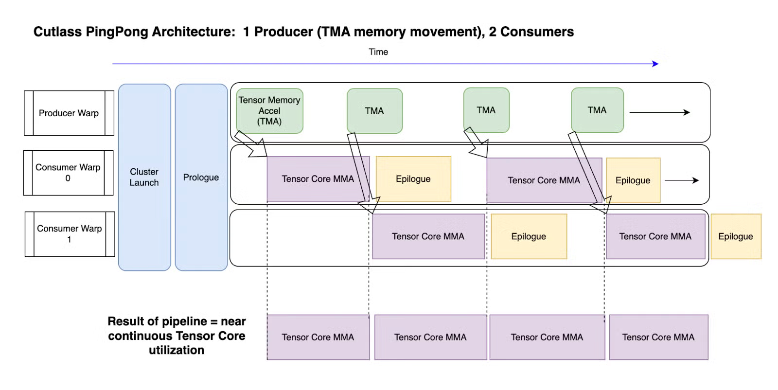 Image extracted from [3].
Cooperative sceduling is almost similar to pingpong scheduling, but both of the consumer warp groups are acting on the same tile, as the tile size might be bigger. To decide when to choose pingpong or cooperative scheduling, there are a few things to consider: Tile size, M dimension, batch size, epilogue complexity, SM pressure, MMA utilization and occupancy etc. If the tile size, or M dimension, or batch size is big, it favours cooperative scheduling, because it gives enough tiles to keep both Warp Groups busy, amortising the Cooperative Synchronization Overhead. If the epilogue is complex, it favours pingpong scheduling, because it can hide the epilogue cost behind next tile’s MMA. Note that if Ping Pong schedule is chosen, the SM pressure would be high because it need more shared memory to store two concurrent tiles.
Some use cases for references:
| Use Case | Recommended | Reason |
|---|---|---|
| Large LLM prefill (large M, large K) | Cooperative | Large tiles, simple epilogue, high arithmetic intensity |
| Batched decode (small M, medium K) | Pingpong | Small tiles, need MMA utilization via overlap |
| Quantized inference fp8 blockwise | Cooperative | Blockwise scaling benefits from large K tiles |
| Fused epilogue (GELU + bias + requant) | Pingpong | Heavy epilogue needs to be hidden behind MMA |
Result and Energy Impact
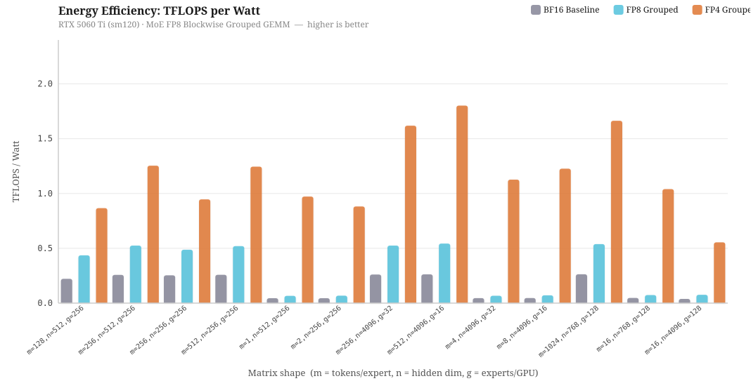 To investigate into the energy efficiency for different kernel implementations, I have ran benchmarks on different configurations of m (tokens/expert), n (hidden dimension) and g (expert / GPU), simulating running of DeepSeek and Qwen model on different Expert Parallelism and Tensor Parallelism configurations. Specifically, even though the number of parameters in a model is the same, increasing the expert parallelism across multiple GPUs will decrease the g, and increasing the Tensor Parallelism will decrease the hidden dimensions, n, by a factor of TP degree.
The chart above benchmarks three kernel implementations — BF16 baseline, FP8 grouped, and FP4 grouped, measured in TFLOPS per Watt on the RTX 5060 Ti at its 180W TDP. Overall, we can see that FP4 grouped kernel has the highest energy efficiency, followed by FP8 grouped, and BF16 baseline. The most interesting insight is when m is small, both FP16 and FP8 grouped kernels perform badly, with FP8 sometimes has equivalent performance compared to the baseline of FP16. This is because when there are few tokens in a batch, there aren’t enough MMA operations to keep the SM occupied, so the GPU spends more time idle relative to the work it is doing, thus low sm occupancy and low throughput per watts. When m is large, all of kernel performance is relatively better than other computation as it has reaches compute-bound. This means that choosing the precision in quantization alone is not sufficient, but batching strategy is also equally important. A deployment running FP8 at low batch size may actually be equally energy efficient than FP16 baseline.
Furthermore, to investigate into the loss in accuracy due to quantization, I have compare FP4 and FP8 numerical accuracy compared to FP16 baseline, and has a surprising discovery. Averaging across benchmark runs, FP4 has 99.10% of cosine similarity to FP16 baseline, while FP8 has 98.14% of cosine similarity to FP16 baseline.
| Metric | FP8 Grouped | FP4 Grouped |
|---|---|---|
| CosSim (↑ better) | 0.9814 | 0.9910 |
| RelRMSE (↓ better) | 0.1978 | 0.1343 |
| Max Abs Error (↓ better) | 97.67 | 55.07 |
Counterintuitively, more bits per element does not automatically mean better numerical accuracy, at least from my empirical studies. My hypothesis is that on my 5060Ti, FP4 uses very fine-grained blockwise scaling factors, thus the dequantization step can very precisely capture the original magnitude in FP16. On the other hand, FP8 uses coarser scaling factor, so while each individual has more bits and range, the overall dequantization step is less precise. If the hypothesis holds, it suggests that scaling granularity may matter more than bit-width for quantization accuracy in LLM inference.
Conclusion
This blog consists of many random notes while I was exploring SGLang repository and cutlass, and many random topics from C++/Python bindings, compiler stack, kernel optimization, quantization etc. I reckon that this blog might be a bit messy, a bit ambitious to cover so many topics, and perhaps a bit shallow in depth due to the scope, but research itself is always entangled with so many topics, and it is always a beautiful journey while I attempt to argue in clarity.
Learning LLM inference and integrating it with energy efficiency concepts is important yet ambiguous. There are many trade offs to consider, many choices to select, and many unknowns to explore. I think I am currently just scratch the tip of a huge iceberg, but I hope this blog offers some valuable insights to you, or tomy future self.