Optimizing Scientific Applications on HPC Systems

Section I - Introduction: The Performance Challenge

Back in the days when single-core processors were the mainstream, software developers enjoyed performance gains every single year thanks to the increase in the number of transistors described in Moore’s Law. These days, Moore’s Law slowly loses its magic as the number of transistors cannot be increased indefinitely because of power constraints. Sometimes, making a bigger integrated circuit by overcoming all the constraints is possible, but it is more expensive, so developers have shifted to multi-core approach (CPU), and more recently massively parallel processors (GPU). As we observe this shift, software engineers who were previously developing single process applications can no longer exploit multi-core CPU or massively parallel GPU benefits without any code changes. This is where the knowledge of parallel programming comes in. Through parallel programming, we engage in iterative optimization cycle: 1. Computing code with parallel programming extension, 2. Profiling the application to identify the bottlenecks and hotspots, 3. Refining the implementation based on profiling insights to reduce execution time and energy consumption. Given the high failure rare to re-design software from scratch, developers typically favor the incremental approach, gradually porting computationally intensive section of code through this continuous feedback loop. In my opinion, this action of code porting in high performance computing (HPC) requires extensive domains of knowledge to excel, including domain knowledge (like physics, biology or chemistry), hardware and software understanding, which makes HPC interesting to learn.

Section II - Understanding Your Scientific Workload

In life, I am a strong believer and advocate for First Principle Thinking, which means to break down problem into its most basic building blocks, then build solutions from those fundamental elements. To me, it goes the same with Performance Optimization for Scientific workload. In this blog, our focus is on GROMACS – a package to simulate molecular dynamics. This focus poses two important questions:

1. What exactly is GROMACS doing?
2. What are the different ways to parallelize GROMACS?

What exactly is GROMACS doing?

GROMACS is a package to enable molecular dynamics simulation of biomolecules like proteins, nucleic acids, and lipids. The simulation could sometimes take a whole day or a whole week depending on the aims of the researchers. An example of the workflow looks like this: 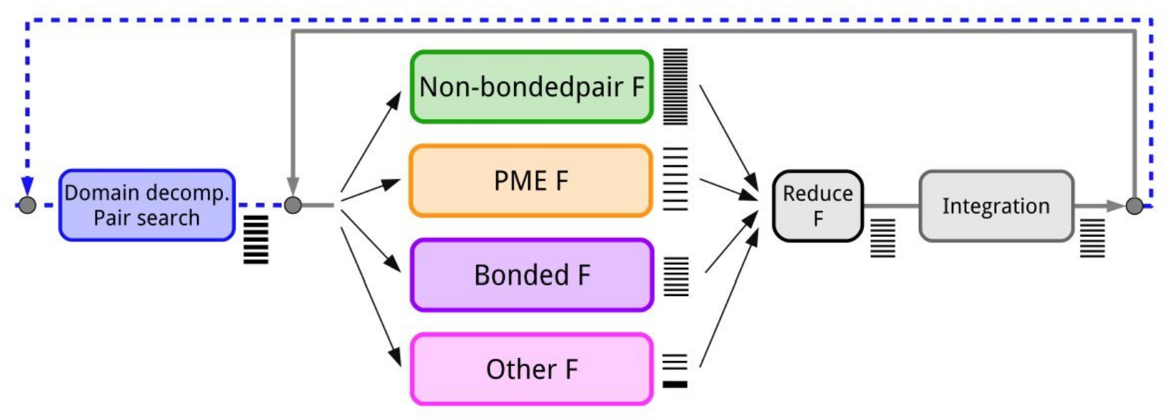Image [1] Source: Páll et al., J. Chem. Phys. 153, 134110 (2020)

Step 1: Domain Decomposition and Pair Search
Domain Decomposition is a way to divide a big domain to smaller domains so that they can be distributed to different processors. While pair search is the process of finding all neighbouring atoms that are within the cut-off distance. As most interactions in molecular simulations are local, domain decomposition is the way to decompose the system to achieve parallelism. As we do that, 2 choices have to be made:

1. The division of a unit into domain
   The division occurs by a default number of units. Note that sometimes when the domain is small, the decomposed domain could be too small for a processor to compute, then the application will throw a warning and halt the run.
2. The assignment of the forces into domains
   After finding the neighbouring atoms and have the neighbour list, we have to let the processors know which forces between the atoms they are responsible to compute. For example, atom A lies in domain boundary of X has force of interaction with another atom B that lies in domain boundary of Y, which domain should be responsible for the force calculation, or perhaps both? The decision making process not only affects the amount of computation, it also affects the communication load as domains have to send each other data to compute the force result. There are three common types of force assignment for atoms near domain boundaries: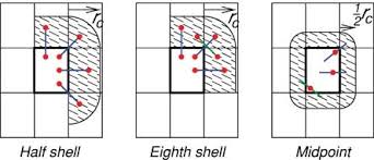 Image [2] Source: Larsson et al., WIREs Comput. Mol. Sci. 1, 93 (2011)

Half shell - In half-shell method, interactions between atoms i and j are computed at the process responsible for atom i or j.
Eighth shell (Used by GROMACS) - In eighth shell method, interactions are distributed among processors such that each processor calculates forces with particles from up to 8 neighboring processor regions (corresponding to the 8 spatial directions: N, NE, E, SE, S, SW, W, NW), with careful coordination to avoid redundant calculations.
Midpoint - In mid-point method, the interaction between i and j is computed by the process which owns the geometric mid-point of i and j.

Step 2: Forces Calculation
Referring to Image [1], in forces calculation, they are independent of each other and can be calculated parallely. The types of forces are as follows:

• Non-bonded forces act between atoms that are not directly connected with chemical bonds. For example, Van deer Waals and Electrostatic force. This is typically N^2 and it scales with the number of atoms.​
• Bonded forces act between atoms and maintain the structure of atoms through covalent bonds, bond angles and dihedral angles.​
• Particle Mesh Ewald (PME) is an algorithm to efficiently calculate the electrostatics forces. PME splits the calculations into long range and short range components using Fourier transform on a grid.

Insight #1: Non-bonded forces is usually the bottleneck in single node setting, 
but PME overtakes non-bonded forces in multinode setting and require more time to complete 
due to communication overhead. The is because PME needs Fast Fourier Transform 
(FFT) to handle the long-range electrostatic interaction calculation. 
And FFT scales poorly in multinode setting. [1]

Step 3: Forces Reduction
Force reduction helps to sum up all overlapping force contributions from the previous steps.

Step 4: Integration
During integration, the application updates the position of atoms by referring to the total force calculated in step 3.

What are the different ways to parallelize GROMACS?

GROMACS offers option on different ways to distribute the workload. A common way is to offload the computationally intensive non-bonded forces calculation to GPU, perhaps together with bonded forces to increase the overall speed up. Domain decompostion and pair search are usually executed in CPU because the overhead of moving them to GPU makes the process inefficient. 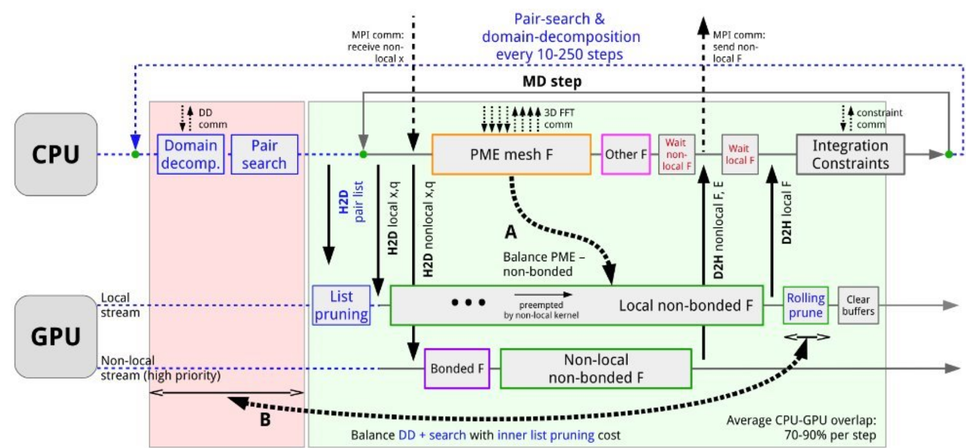Image [3] Source: Páll et al., J. Chem. Phys. 153, 134110 (2020)

The diagram above illustrates the parallelization strategy in GROMACS. CPU is responsible for domain decomposition and pair search, integration and sometimes PME mesh force if the FFT library is CPU based. Meanwhile, GPU is responsible for non-bonded forces and bonded forces. In the timeline, there are 70-90% CPU-GPU overlap per step.

The following image shows other ways of offloading.
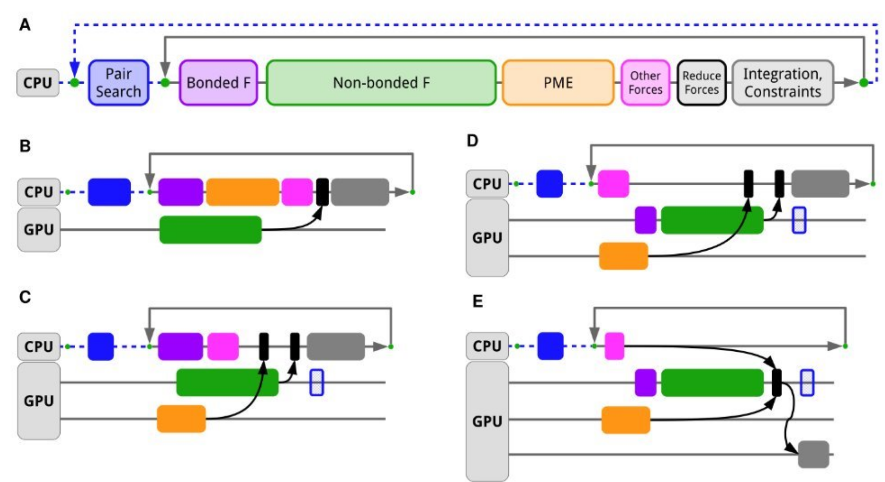Image [4] Source: Páll et al., J. Chem. Phys. 153, 134110 (2020)

Section III - Hardware-Level Optimization Strategies

Hardware level understanding are usually inseparable in order to perform good optimization. Things like cores, cache hierarchy and coherence, NUMA, RDMA and NIC, and CUDA-aware MPI are essential in HPC understanding. Let’s break it down one by one:

Cores

In computing, a core refers to an individual processing unit within a CPU. In HPC, it is common to observe multiple cores within a socket, and dual-socket architecture designs are also prevalent in high-performance CPU servers. This hierarchical design has been developed further by implementing different memory architectures to exploit the locality in memory access that appears in many applications.

Cache hierarchy and coherence

Cache hierarchy is a product of the trade-off between cost and speed. It bridges the speed gap between the processor and main memory, thereby improving overall system performance.

Cache coherence is required in multi-processor systems where multiple processors have their own caches that may contain copies of the same memory locations. It is essential in multi-processor systems to ensure data consistency across multiple caches and main memory. Some protocols used in cache coherence include MSI and MESI (Modified, Shared, Invalid and Modified, Exclusive, Shared, Invalid, respectively).

NUMA

When we have distributed memory, we operate under NUMA (Non-Uniform Memory Access) architecture, where memory access times are non-uniform. Imagine a system with multiple sockets, each with its own DRAM, connected through an interconnect. The key principle is that CPU 1 has higher bandwidth to DRAM 1, and CPU 2 has the same high bandwidth to DRAM 2. However, cross-socket access (CPU 1 to DRAM 2) incurs higher latency and lower bandwidth. In essence, under NUMA, a processor can access its own local memory faster than non-local memory. NUMA is beneficial for workloads with high memory locality because it reduces traffic on the memory interconnect and improves overall system performance.

RDMA

While NUMA is a computer memory design used in multiprocessing that optimizes memory access within a single multi-processor system, RDMA is a network-based remote memory access technology. RDMA allows nodes to directly access memory on remote machines, enabling high-performance communication between different computers over a network. It works by bypassing the CPU and operating system to directly transfer data between the memory of different machines, thereby reducing latency and CPU overhead for inter-node communication.

NIC

NIC is the Network Interface Card, a physical hardware that connects a computer to a network, and is closely related to both NUMA and RDMA in modern HPC system. It handles the transmission and reception of data packets over network connection (Ethernet, InfiniBand, etc). By having NIC, it allows data to reside in network buffer, which ideally should be allocated in the same NUMA node as the NIC to minimize cross-NUMA traffic.

In scientific computing, halo exchange (also called ghost cell exchange) is a critical concept that NICs help solve efficiently. In application like GROMACS, when we decompose a computational domain, each processor works on a subdomain. However, the boundaries must be exchanged because calculations at the boundary of one subdomain often depend on data from neighboring subdomains.

Traditioinal Ethernet-based communication requires significant CPU involvement for managing network protocols and data transfers, which leads to high latency for small boundary data transfer and CPU overhead for managing many small communications. NIC helps with halo exchange by having minimal CPU involment, at the same time, NIC enable direct remote memory access for ghost cell updates, essentially allows computation-communication overhead. In short, it is a smart buffer manager that handle the frequent boundary data exchange, so that CPU focuses on computation.

CUDA-aware MPI

CUDA-aware MPI is the programming interfaces that leverage all three NIC, RDMA and NUMA. This example below from NVIDIA’s blog shows how CUDA-aware MPI helps to reduce staged communication.

• Without CUDA-aware MPI

//MPI rank 0
cudaMemcpy(s_buf_h,s_buf_d,size,cudaMemcpyDeviceToHost);
MPI_Send(s_buf_h,size,MPI_CHAR,1,100,MPI_COMM_WORLD);

//MPI rank 1
MPI_Recv(r_buf_h,size,MPI_CHAR,0,100,MPI_COMM_WORLD, &status);
cudaMemcpy(r_buf_d,r_buf_h,size,cudaMemcpyHostToDevice);

• With CUDA-aware MPI

//MPI rank 0
MPI_Send(s_buf_d,size,MPI_CHAR,1,100,MPI_COMM_WORLD);

//MPI rank n-1
MPI_Recv(r_buf_d,size,MPI_CHAR,0,100,MPI_COMM_WORLD, &status);

From the example, we can see that when we are combining MPI and CUDA, we often need to send GPU buffers instead of host buffers. Without CUDA-aware MPI, we need to stage GPU buffer through host memory, but with CUDA-aware MPI, GPU memory allocated with cudaMalloc can be used directly in MPI calls. The key technology behind it is GPUDirect RDMA, where MPI buffer transfer are done directly from GPU to GPU whenever possible, without an intermediate copy on the CPU memory.

In GPU-accelerated scientific application, halo exchange can happen directly between GPU memories across nodes, making the boundary updates much more efficient. Besides, modern implementation often combine CUDA-aware MPI with RDMA-capable NIC to achieve the lowest possible latency for GPU-to-GPU communication.

Section IV - Software Stack Optimization

Library selection (MKL, OpenBLAS, FFTW, CuFFT, CuFFTMp)

In high-performance molecular dynamics simulations, the choices of mathematical libraties can severely impact the performance. For instance, GROMACS relies heavily on optimized implementation of linear algebra (BLAS/LAPACK) and Fast Fourier Transform (FFT).

Basic Linear Algebra Subprograms (BLAS) and Linear Algebra (LAPACK) form the backbond of many scientific computations, handling matrix operations, eigenvalue problems, and linear system solving. These packages usually will have extensive tiling method, optimized memory movement, and caching that optimize the performance. Meanwhile, FFT libraries are essential for PME calculations, which dominates the computational cost in large biomolecular system.

CPU-Optimized Libraries

1. Intel Math Kernel Library (MKL)

• Intel MKL is highly optimized for Intel processors with architectural awareness.
• They have automatic dispatch to processor-specific code paths (SSE, AVX, AVX512)

2. OpenBLAS

• Open-source alternative that is offering good performance across different architectures (Even AMD and ARM processors)
• Often preferred in heterogeous computing environments.

3. FFTW3

• Gold standard for CPU-based FFT operations
• GROMACS developers’ recommended choice for CPU FFT operations.

GPU-Accelerated Libraries

1. cuFFT (CUDA FFT Library)

• NVIDIA’s optimized FFT implementation for single-GPU systems
• Excellent performance for moderate scale simulations but limited to single-node GPU configurations

2. cuFFTMp (multi-process cuFFT)

• Multi-GPU extension of cuFFT for distributed memory system

3. VkFFT

• FFT library with broad hardware support, allow cross platform compatibility.
• Increasingly adopted for heterogenous computing environments.

The key insight is that optimal library selection must consider not just computational efficiency, but also how well the library integrates with the underlying network topology and memory architecture - connecting directly to our earlier discussions of NUMA awareness and RDMA optimization.

Scaling Issue with 3D FFT

In GROMACS molecular dynamics simulations, 3D FFT are critical for computing long range electrostatic interactions through the Particle Mesh Ewald (PME) method. The PME algorithm is essential for accurate modeling of forces in biomolecular symtems, but presents significant scalability challenges. The picture below shows the flow of 3D FFT as an example: 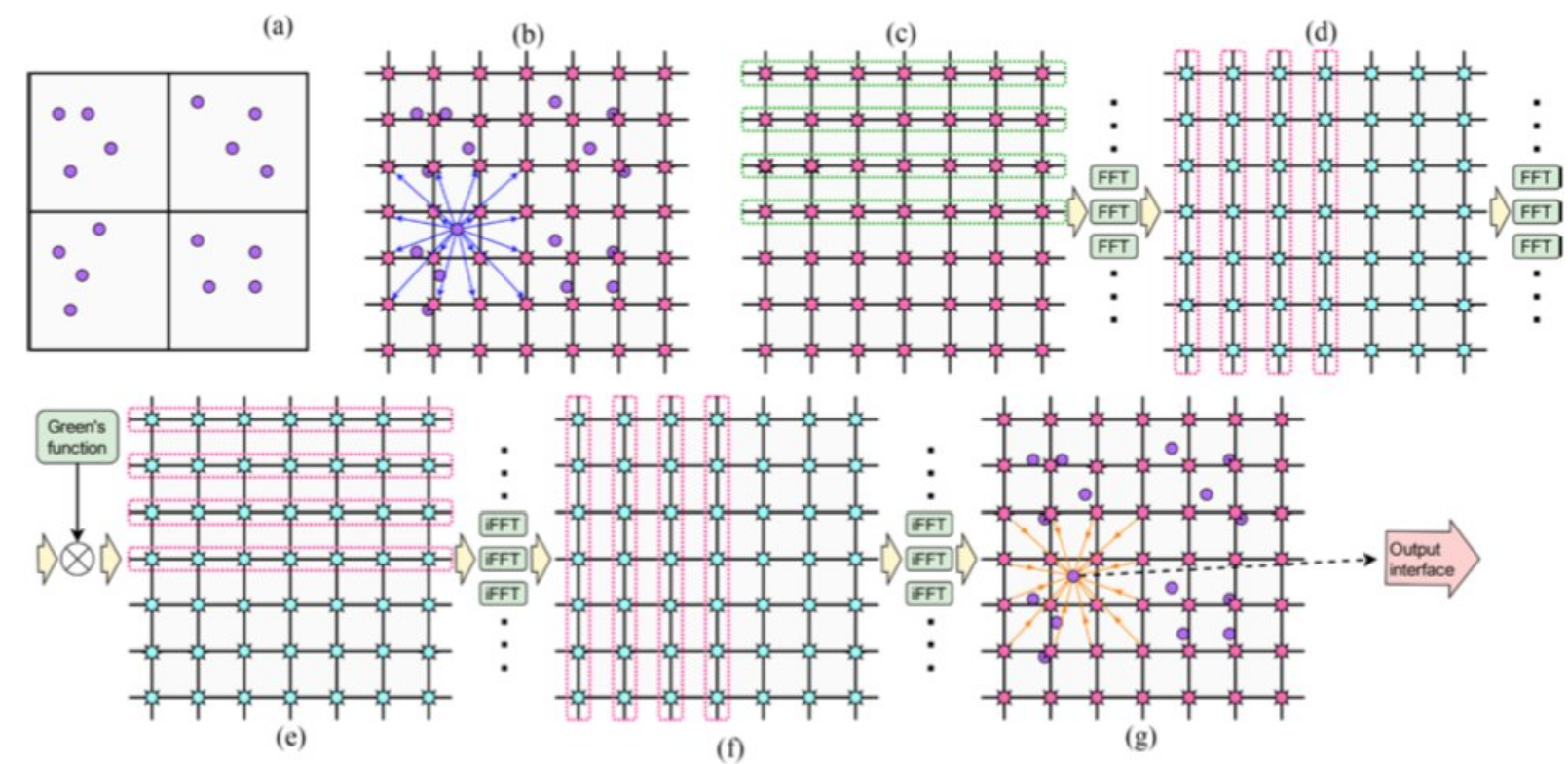Image [5] Source: Bandara et al.: Long-range MD Electrostatics Force Computation on FPGAS​
Firstly, (a) shows particles in a simulation space, organized into calls, as needed for computation. Then, (b) shows the first step in PME, which is to distribute the charge of a particle onto a charge grid. Subsequently, (c) and (d) performed FFT in separate steps. (e) and (f) do multiplication and inverse FFTs. Lastly, (g) shows the forces from 64 nearby grid points being applied to a particle.

One must be wondering why do we need FFT in calculating PME. FFTs allow for a rapid transformation of charge density information from real space to a spectral or reciprocal space, where the Poisson equation (solving for electrostatic potential) becomes a simpler algebraic problem. After solving in reciprocal space, an inverse FFT is used to transform the potential back to real space.​ So essentially, FFT is helping us to calculate whats hard to calculate in real space, by transforming the charge density information to reciprocal space, where the calculation is easier to perform.

However, the FFT scalability is notoriously bad. According to the research performed by Oak Ridge National Lab and University of Manchester, MPI communication accounts for 97% of the processing time when we weak scale (constant problem size per processor) heFFTe (GPU) on 1024 Summit nodes. This communication overhead has caused the performance to deteriorated. Here, we found that the bottleneck isnt the computation, but its about moving the data efficiently between nodes, which is why understanding the interconnect technologies (NICs, RDMA, etc) is so crucial for HPC application like GROMACS.

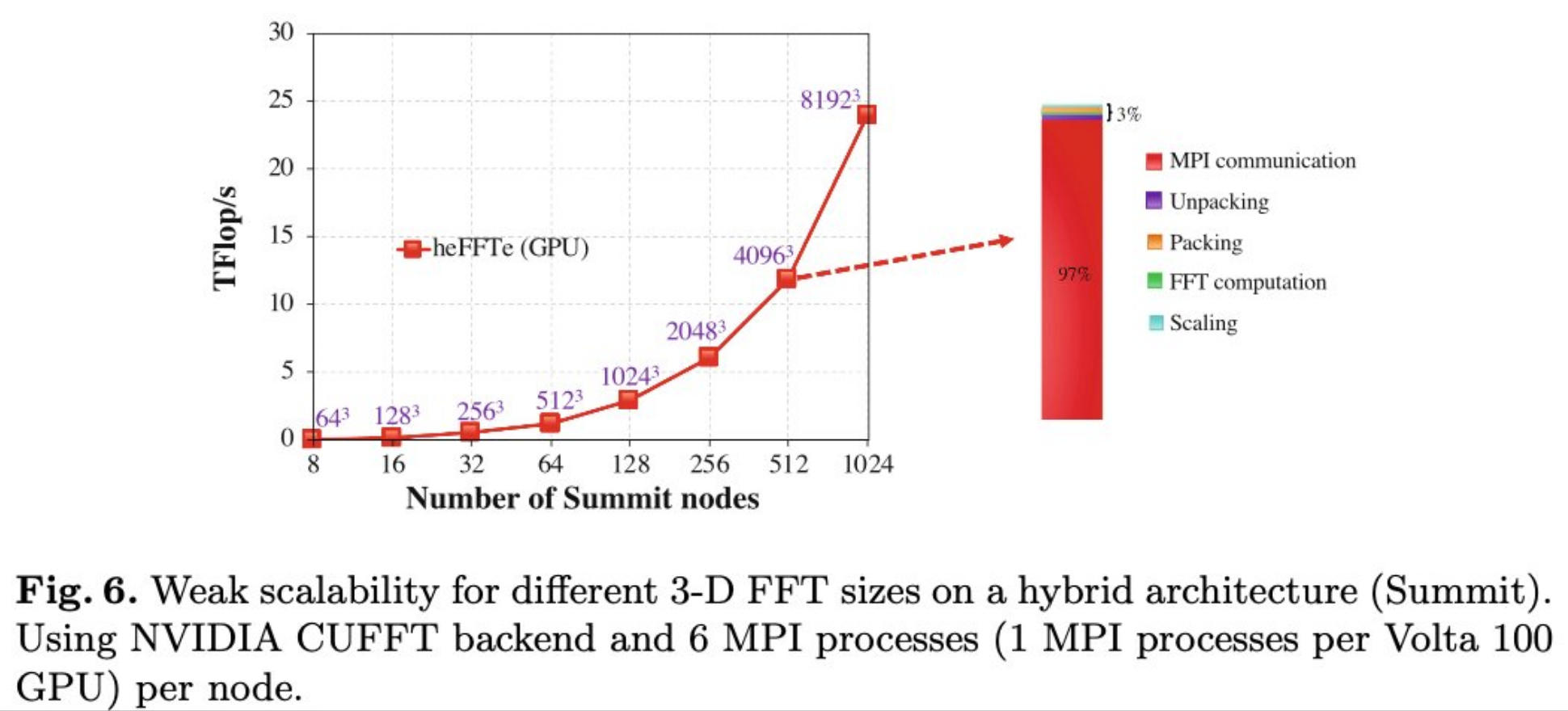Image [6] Source: Ayala et al.: Scalability Issues in FFT Computation

Section V - Green Computing

As the need for computing power increases over the years, one important factor that we have to consider is energy. Energy consumpstion is also one of the driving forces that push Singapore to have the first deployment of warm water cooling system in a tropical environment. The innovative cooling system helps to achieve high performance, and at the same time save energy. Zooming out from the big picture, when we look at performance optimization, energy consumption is also an important factor when we are selecting which architecture to use.

For GROMACS, we might be wondering whether it is CPU or GPU that consumes lesser energy. If it is CPU, which architecture? If it is GPU, which generation? In our experiment, we use Intel’s Running Average Power Limit (RAPL) interface to report the energy consumption, and nvidia-smi to sample the average power usage for each run. Besides, we use three different dataset to benchmark the performance, which are MD_15NM_WATER, STMV, HecBioSim3M, with 300k, 1M, and 3M respectively.

In essence, the question that we are trying to solve is:

Is GROMACS greener on CPU or GPU on ASPIRE2A?

The results:

Which is greener? CPU or GPU on ASPIRE2A? – GROMACS 2025

Platform: ASPIRE 2A

Dataset: MD_15NM_WATER (300k atoms)

Config	Performance (ns/day)	Average kW Power per second (Total CPU + GPU)	Total Energy (kWh: Power x Time)	SU Credits	Perf/Average kW Power
4 CPU Nodes	135.3	1.705	0.02558	7.68	79.35
8 CPU Nodes	There is no domain decomposition for 896 ranks that is compatible with the given box and a minimum cell size. STMV system is still too small for 896 MPI ranks
2 GPU Cards - CUDA	178.5	0.5063	0.001051	1.049	352.6
2 GPU Cards - SYCL	63.34	0.4593	0.006226	2.122	137.9
4 GPU Cards - CUDA	191.7	0.8452	0.001108	1.998	224.9
4 GPU Cards - SYCL	75.81	0.5967	0.008112	7.936	127.0

Dataset: STMV (Satellite Tobacco Mosaic Virus) - 1 Million atoms

Config	Performance (ns/day)	Average kW Power per second (Total CPU + GPU)	Total Energy (kWh: Power x Time)	SU Credits	Perf/Average kW Power
4 CPU Nodes	25.63	1.953	0.07922	20.76	13.12
8 CPU Nodes	There is no domain decomposition for 896 ranks that is compatible with the given box and a minimum cell size. STMV system is still too small for 896 MPI ranks
2 GPU Cards - CUDA	37.64	0.6142	0.01689	3.498	61.28
2 GPU Cards - SYCL	23.33	0.5728	0.02100	5.546	40.73
4 GPU Cards - CUDA	60.27	1.019	0.01443	7.936	59.15
4 GPU Cards - SYCL	33.64	0.8526	0.02747	8.064	39.46

Dataset: HECBioSim (A Pair of hEGFR tetramers of 1IVO and 1NQL) - 3 Million atoms

Config	Performance (ns/day)	Average kW Power per second (Total CPU + GPU)	Total Energy (kWh: Power x Time)	SU Credits	Perf/Average kW Power
4 CPU Nodes	9.975	1.960	0.1938	50.63	5.089
8 CPU Nodes	17.98	1.946	0.2386	62.86	9.239
2 GPU Cards - CUDA	7.382	0.4937	0.02488	16.85	14.95
2 GPU Cards - SYCL	5.626	0.5677	0.07302	22.06	9.910
4 GPU Cards - CUDA	18.47	1.035	0.05118	17.84	17.84
4 GPU Cards - SYCL	10.17	0.8956	0.07787	26.33	11.26

Key Findings

1. GROMACS is “greener” on GPU

   • GPU configurations consistently achieve better performance-to-power ratios compared to CPU-only setups

2. Multi-node CPU consumes more power than Single Node GPU

   • 4 CPU nodes consume 1.705-1.960 kW compared to 2 GPU cards at 0.4937-0.6142 kW
   • GPU solutions deliver comparable or superior performance with dramatically lower power consumption

3. Which GPU config is greener? It depends on the problem size

   • <1M atoms: Use 2 GPU cards (optimal efficiency: 352.6 and 61.28 perf/kW for 300k and 1M atoms respectively)
   • >1M atoms: Use 4 GPU cards (17.84 perf/kW for 3M atoms provides better scalability)

4. CUDA implementation outperforms SYCL

   • CUDA consistently shows better performance than SYCL implementation across all system sizes
   • This is because CUDA tmpi code is optimize with GPU Direct, but SYCL tmpi code is not, so to be fair this is a comparison of direct communication vs staged communication, but not CUDA vs SYCL.

5. Limitations on Power Measurement

   • Nvidia-smi only measures chip power, excluding GPU board components (memory, fans, other components)
   • Measurements exclude power consumption from memory, network, storage, and I/O subsystems
   • Actual total system power consumption may be higher than reported values
   • Results should be interpreted as relative comparisons rather than absolute power consumption

With our existing system, we are also interested in this question:

Shoudl we use A100 or H100 for GROMACS?

The result:

Which is faster? ASPIRE 2A (A100) vs ASPIRE 2A+ (H100) for GROMACS.

Dataset: MD_15NM_WATER (300k atoms)

Config	ASPIRE2A A100 Performance (ns/day)	ASPIRE2A+ H100 Performance (ns/day)	Speed Up
2 GPU Cards - CUDA	178.5	283	1.58
2 GPU Cards - SYCL	63.34	107	1.69
4 GPU Cards - CUDA	191.7	375	1.96
4 GPU Cards - SYCL	75.81	90.4	1.19

Dataset: STMV (Satellite Tobacco Mosaic Virus) - 1 Million atoms

Config	ASPIRE2A A100 Performance (ns/day)	ASPIRE2A+ H100 Performance (ns/day)	Speed Up
2 GPU Cards - CUDA	37.64	64.9	1.72
2 GPU Cards - SYCL	23.33	43.6	1.87
4 GPU Cards - CUDA	60.27	126.1	2.09
4 GPU Cards - SYCL	33.64	49.9	1.48

Dataset: HECBioSim (A Pair of hEGFR tetramers of 1IVO and 1NQL) - 3 Million atoms

Config	ASPIRE2A A100 Performance (ns/day)	ASPIRE2A+ H100 Performance (ns/day)	Speed Up
2 GPU Cards - CUDA	7.382	17.19	2.33
2 GPU Cards - SYCL	5.626	11.81	2.10
4 GPU Cards - CUDA	18.47	28.09	1.52
4 GPU Cards - SYCL	10.17	12.34	1.21

Key Findings: A100 vs H100 for GROMACS

1. H100 consistently outperforms A100 across all configurations

   • Speed improvements range from 1.19x to 2.33x depending on system size and configuration

2. The results are consistent with what NVIDIA has published

   • (https://developer.nvidia.com/hpc-application-performance)

3. Recommendation: Choose H100 (ASPIRE 2A+)

   • Significant performance improvements across all tested scenarios

Power Measurement: Intel-rapl and Nvidia-smi

Section VI - Profiling and Performance Analysis

Performance Modeling

Roofline Model

In performance modeling, roofline model is famous for its intuitive visual explanation of performance estimates of a given kernel or application that is running on multi-core CPU or accelerators like NVIDIA GPU. In practice, it uses microbenchmarks to compute peak performance of a machine as a function of arithmetic intensity (a performance metrics that describes the ratio of computation to memory access in a program) of application, then compare application’s performance to known peak values. An example of the graph is shown here: 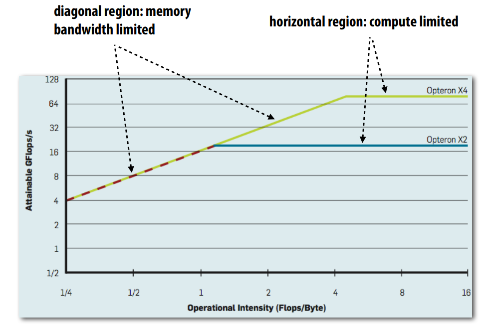Image [7] source: Willians et al. 2009 and Standford Parallel Computing Lecture 6

In the image above, the diagonal region shows memory bandwidth limited performance. In this region, when we increase the operational intensity by having more computation per memory byte transfered, the performance increases linearly because the application is constrained by how quickly data can be moved from memory to the processor. The diagonal region is exclusively memory bound, which means the processor has sufficient computational capabity, but performance is limited by memory bandwidth.

When the operational intensity increases enough to reach the horizontal region, the application becomes compute bound. At this point, the program is no longer limited by memory bandwidth, but instead constrained by the processor’s computational throughput. A further increase in operational intensity will not improve performance because the processor has reached its maximum computational capacity.

If a research engineer is interested to profile this graph, one can use NVIDIA's Nsight Compute to profile the kernel. After that, there are various levels of optimization that can be performed to improve the performance. For instance:

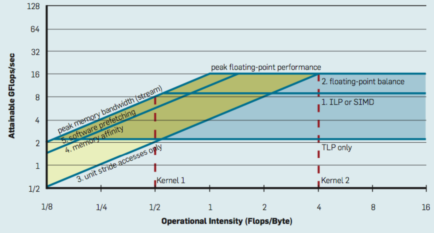Image [8] source: Willians et al. 2009 and Standford Parallel Computing Lecture 6

Compute vs memory vs I/O bound

Other than compute and memory bound, we also have I/O bound. In reality, we can’t really have one application to have only one specific type of bound. Often, it is a mixed scenarios where scientific application exhibit different bottlenecks during different phases. For example:

• Climate models could be compute bound during physics calculations, but I/O bound during checkpointing for each time stamp
• Molecular dynamics simulations are typically compute-bound during force calculations (electrostatic, van der Waals interactions) and communication-bound (MPI-bound) due to frequent halo exchanges and domain decomposition communication between processes.

System-Wide Profiling - nsys, ipm, arm-forge

For system-wide profiling, there are several tools that can be used. When we do system wide profiling, instead of diving deep, we actually take a step back and look at the overall performance. For example: We look into how CPU and GPU works together, whether there’s GPU peer-to-peer memory transfer, whether there’s NVTX to explain the CPU activity, etc.

A wide range of tools that can be considered: nsight, ipm, arm-forge.

• nsight is the go-to profiler that we will use for GPU application, it provides information like memory transfer, most computatioinally intensive kernel, and sometimes NVTX to explain CPU activity.
• ipm is the portable profiler that was prebuilt and included in older versions of HPC-X (note that it has been removed for the latest version, but personally I find it qutie useful). IPM records communication sorted by rank, gives you information about the types of MPI functions used and communication topology.
• arm-forge or linaro-forge reveals application activity, CPU floating-point information and memory usage, but it requires license in order to use it.

NVIDIA Nsight System

An example of using Nsight System to profile GROMACS - 4 GPU cards within a node (CUDA backend) in ASPIRE2A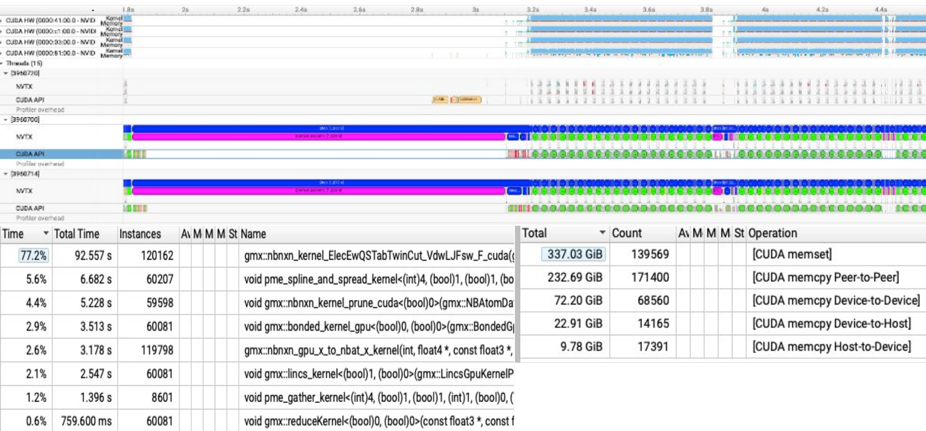： In here, we revealed that non-bonded kernel is the most computationally intensive kernel, and CUDA memcpy Peer-to-Peer exists which means that GPU Direct is being used.

IPM

An example of using IPM to profile GROMACS - 1 CPU node in ASPIRE2A: 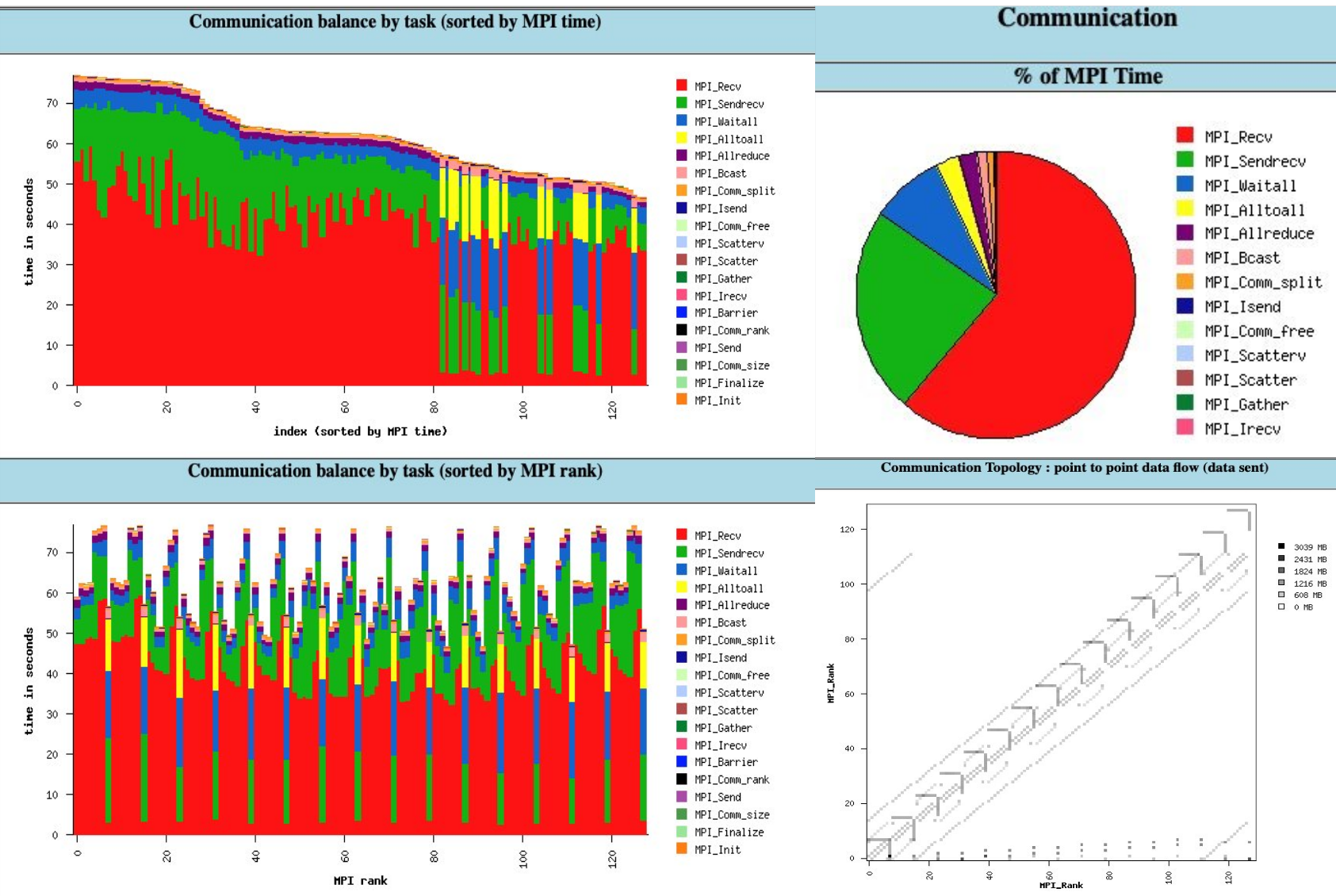In IPM with CPU setting, we understand that there are many point-to-point communication, a few all to all / all reduce and Bcast.

In the communication topology, main diagonal line exposes neighbor-to-neighbor communication (Short Range Interaction – van der Waals, electrostatics within cutoff) - (pp, Rank 0-6)​. Meanwhile, horizontal/vertical Lines are collective communication pattern (Long Range Electrostatic, Constraint) - (pme, Rank 7)​. Also, for every 8 ranks, there will be 1 rank focusing on all-to-all broadcast, for collective communication.

Arm-forge or Linaro-forge

An example of using Arm-forge to profile GROMACS - 1 CPU node in ASPIRE2A:

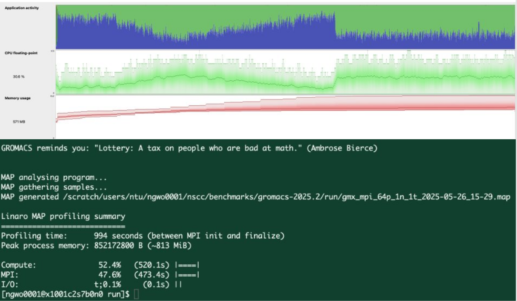
In linaro forge, we understand that I/O is not the bottleneck. While Compute and MPI communication is 50/50 at this scale. (1 CPU Node with 128 ranks)

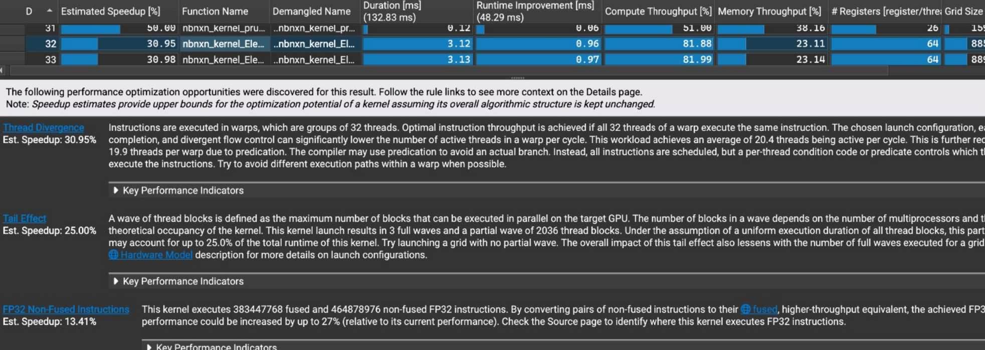
Kernel-Level Profiling - ncu

NOTE: ncu enable kernel level profiling, but it requires GPU performance counter, hence user-level might not be able to execute it
An example of memory access patterns and cache performance of a GPU kernel execution: 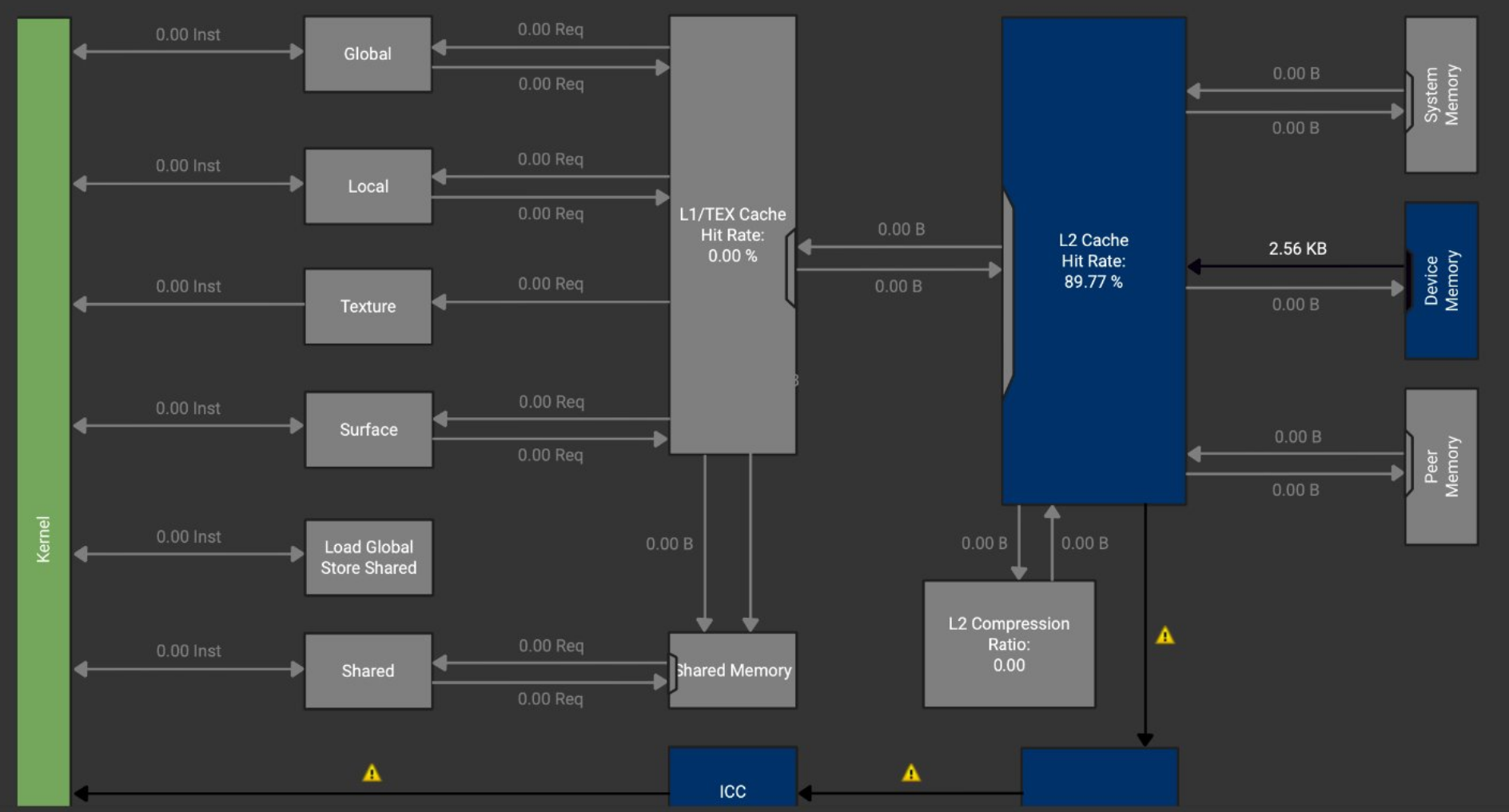Optimization recommendations for CUDA kernels

Section VII - Automation and Reproducibility

For automation, we choose spack to automate the build process in order to achieve reproducibility. Spack is a package manager for supercomputers, and it aims to make installing scientific software easy. A sample script that I have used on ASPIRE2A is shown here:

cd scratch
git clone --depth=2 --branch=releases/v0.23 https://github.com/spack/spack.git
cd spack

# Source the setup script to initialize Spack environment
# This adds Spack commands to your shell environment
. share/spack/setup-env.sh

# List available packages (gromacs appears in the output)
spack list

module purge
module load gcc/13.3.0    
module load cmake         
module load cuda/12.6.2   
module list

# Set Spack cache directory and create it
export SPACK_USER_CACHE_PATH=~/scratch/spack/cache
mkdir -p ~/scratch/spack/cache

# Find available compilers in the system
spack compiler find

# Configure Spack to use specific compiler and MPI with CUDA support
# [email protected]: Install GROMACS version 2024.3
# ~mpi: Disable MPI support
# +cuda: Enable CUDA support
# cuda_arch=90: Target CUDA compute capability 9.0 (for newer GPUs)
spack compiler spack spec [email protected] ~mpi +cuda cuda_arch=90

# Find external packages that Spack can use instead of building from source
spack external find cuda    
spack external find cmake   
spack external find gcc make autoconf automake libtool bison perl pkg-config
spack external find m4 tar zstd bzip2 pkg-config xz openssl gmake

# Show the dependency tree and build plan for GROMACS
spack spec [email protected] ~mpi +cuda cuda_arch=90

# Install GROMACS with the specified configuration
spack install [email protected] ~mpi +cuda cuda_arch=90

# Find and load the installed GROMACS package
spack find -p gromacs

To manage the package dependencies, we can edit /home/user/<institution>/<username>/.spack/packages.yaml. This file in Spack allows us to configure external packages that are already installed on the system, set preferred versions of software packages, set build preferences and compiler options.

Citation

1. Ayala, A., Tomov, S., Stoyanov, M., & Dongarra, J. (2021, September). Scalability issues in FFT computation. In International Conference on Parallel Computing Technologies (pp. 279-287). Cham: Springer International Publishing.
2. Bandara, S., Ducimo, A., Wu, C., & Herbordt, M. (2024). Long-Range MD Electrostatics Force Computation on FPGAs. IEEE Transactions on Parallel and Distributed Systems.
3. Larsson, P., Hess, B., & Lindahl, E. (2011). Algorithm improvements for molecular dynamics simulations. Wiley interdisciplinary reviews: computational molecular science, 1(1), 93-108.
4. Páll, S., Zhmurov, A., Bauer, P., Abraham, M., Lundborg, M., Gray, A., … & Lindahl, E. (2020). Heterogeneous parallelization and acceleration of molecular dynamics simulations in GROMACS. The Journal of chemical physics, 153(13).
5. Williams, S. W., Waterman, A., & Patterson, D. A. (2008). Roofline: An insightful visual performance model for floating-point programs and multicore architectures (Vol. 1). Technical Report UCB/EECS-2008-134, EECS Department, University of California, Berkeley.
6. Andersson, M. I., Murugan, N. A., Podobas, A., & Markidis, S. (2022, September). Breaking down the parallel performance of gromacs, a high-performance molecular dynamics software. In International Conference on Parallel Processing and Applied Mathematics (pp. 333-345). Cham: Springer International Publishing.
7. Hwu, W. W., Kirk, D. B., & Hajj, I. E. (2022). Programming massively parallel processors: A hands-on approach (4th ed.). Morgan Kaufmann.
8. Fatahalian, K., & Olukotun, K. (2024). CS149: Parallel computing [Course]. Stanford University, Department of Computer Science.