Whilst DiT has been around in the AI world for a while, we’ve only recently started catching up with efficient AI systems for this specific use case, for example, LongLive from NVIDIA’s lab. To actually understand its backbone, and before we can speed up the DiT in CuteDSL, let’s understand the architecture first, followed by the math, and lastly, how we can speed it up.
The Architecture
Under LongLive, the architecture is as follows:
 By giving a prompt, we use an encoder to encode the prompt into a representation that the DiT can understand, basically converting a string to a Tensor. After that, the DiT denoises the current latent representation until it reaches a clean state. For each latent frame, the VAE can decode it into 4 video frames, which is 1/6 second at 24 fps. Usually, both DiT and VAE will make up to about 90% of the end-to-end video generation time, with DiT running slightly longer than VAE.
Contrary to how an LLM builds up KV cache in the order of tokens, DiT builds up KV cache from the perspective of a chunk, where each chunk has 8 latent frames, and each latent frame is 880 tokens, total up to 7040 tokens per chunk. The KV cache design is shown as follows:
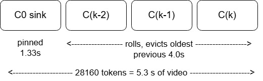 The KV window has 4 KV chunks. For the first chunk, it is the first 8 latent representations that are permanently stored in the KV cache due to the observation of the attention sink, where the first tokens could have contributed a majority of the softmax score [1], also making sure that the video generated by the model doesn’t drift as much as compared to its original prompt intention. Then, a rolling window will cover the most recent 2 chunks, as well as the current chunk. Overall, 5.3 seconds of the video will be cached as KV cache.
The Math in DiT
1. Sampling the noise
The main idea of DiT is to denoise a noisy latent until it reaches its predicted clean state. For each chunk, LongLive implements 5 DiT forwards, where 4 out of the 5 are sampling steps, meaning sampling the noise and trying to denoise it at the same time based on the given prompt, and the last is to rewrite the KV cache into a clean version, so the next chunk can attend to the correct KV values. This is also used in LongLive 1.0 [2] – rewriting the KV cache of clean latent in the fifth pass instead of using the partially noisy one from the fourth.
Regardless, let’s talk about the most important input for DiT – the noisy latent frame is defined as follows:
$$ x_{\sigma} = (1-\sigma)x_{0} + \sigma\epsilon \tag{1} $$where the $\epsilon$ is the Gaussian noise, $\sigma$ is the noise level and $\sigma \in [0,1]$ ($\sigma=0$ is the clean video and $\sigma=1$ is pure noise), and finally, $x_{0}$ is the clean latent state (video) that the model believes is currently hiding under the noise. The idea of DiT is basically trying to find the $x_{0}$ using the minimum number of DiT steps.
More importantly, we need to know how DiT moves the noisy latent representation into the clean one, what does it use to update the latent value? One observation we find is that the target that the DiT model learns, for a given $x_{0}$ and $\epsilon$, is constant regardless of the $\sigma$. Specifically, the derivative, or more commonly the flow, is:
$$ v = \frac{d x_{\sigma}}{d\sigma} = \epsilon - x_{0} \tag{2} $$$v$ is therefore the information that DiT derives in each pass, and will be fed into the noisy latent, and moves it towards the clean latent state. Mathematically speaking, by putting (2) into (1), we have
$$ x_{\sigma} = (1-\sigma)x_{0} + (v+x_{0})\sigma = x_{0} + v\sigma $$and hence
$$ x_{0} = x_{\sigma} - v\sigma \tag{3} $$The idea of DiT is therefore depicted here. The supposedly clean video is approximated by us, using the noisy latent state, as well as the flow predicted by the DiT, set at the current noise level $\sigma$.
2. Denoising the Latent
The denoising of the accurate latent frame can be much more efficient if we calculate the absolute $x_{0}$ in one pass. However, we can’t know the absolute $x_{0}$ in practice because, during the training of DiT, it is trained to approximate the flow $v$ based on the average possible denoised latent frames generated from one noisy latent. Hence, during inference, the correct formula should really be:
$$ \hat{x}_{0} = x_{\sigma} - v\sigma \tag{4} $$where the $\hat{x}_{0}$ will drift as the $\sigma$ changes. A sampler’s job, like UniPC, is therefore to follow the drift with as few DiT passes as possible. Note that in LongLive, the $\sigma$ will change throughout the 5 DiT passes, ranging from [0.9998, 0.9373, 0.8331, 0.6247, 0]. This means the noise level starts extremely high and slowly decreases across passes. One can imagine this as the process of generating an image: from a noisy latent to a blurry background, then to composition, subjects, and finally perhaps sharpness, lighting, and other small details. The pseudocode is as follows (extracted from pipeline/causal_diffusion_inference.py:596–660):
# For a single shot, LongLive generates 48 chunks == 1 minute-ish worth of video
for b in 0 .. 47:
    x = randn(8 frames)   # σ = 1 for all 8 frames
    for σ_i in [0.9998, 0.9373, 0.8331, 0.6247]:
        # self-attn over cached past chunks + this noisy chunk
        v = DiT(x, t = 1000 • σ_i, text, kv_cache)
        x = UniPC_step(v, σ_i -> σ_{i+1}, x)
    # this chunk's x̂₀, later VAE-decoded
    output[b] = x
    # clean forward, overwrite the chunk's K/V
    DiT(x, t = 0, kv_cache, write_cache=True)
    roll the cache if the 4-chunk window is full (sink stays)
3. One DiT block
In DiT, our main motive is to denoise the $x_{\sigma}$ into an approximated clean latent form $\hat{x}_{0}$ through multiple iterations. At the same time, we want to make sure that the produced latent is coherent with our prompt, thus cross attention, and making sense across pixels, thus self attention. As a result, the DiT will take 3 different types of inputs, namely: prompt $p$, the noise level $\sigma$ and the noisy latent $x_{\sigma}$, and output the flow $v$, which will then be fitted into UniPC to produce the estimated $\hat{x}_{0}$, which will then be used by VAE model to produce the final pixels.
$$ \underbrace{p,\ \sigma_i,\ x_{\sigma}}_{\text{inputs}} \ \xrightarrow{\ \text{DiT}\ }\ v \ \xrightarrow{\ \text{UniPC}\ }\ x_{\sigma'}\ \text{(steps 1–3)}\ \ \text{or}\ \ \hat{x}_0\ \text{(step 4)} \ \xrightarrow{\ \text{VAE}\ }\ \text{pixels} $$In each and every DiT block, it consists of several steps, LayerNorm, RMSNorm, QKV Projections, 3D RoPE, KV Cache, Self Attention and Cross Attention. The exact flow can be roughly understood as below.
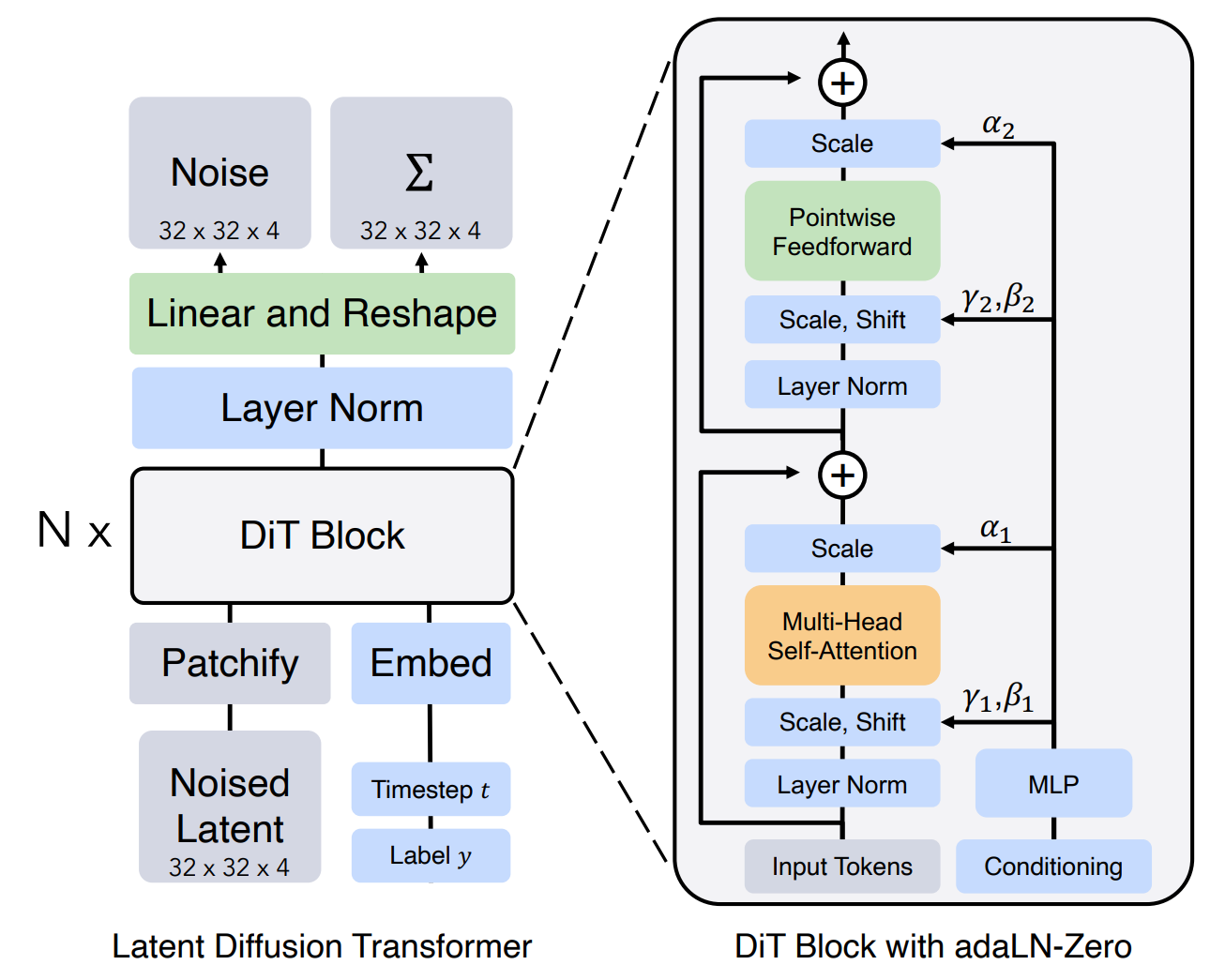 Image is extracted from the DiT Paper [3].
Given the input: prompt $p \ \xrightarrow{\ \text{umT5 + MLP}\ }\ c \in \mathbb{R}^{1\times 512\times 3072}$, noise level $\sigma_i \ \xrightarrow{\ t = 1000\sigma_i,\ \text{sinusoidal + MLP}\ }\ e \in \mathbb{R}^{1\times 8\times 3072}$, and the noisy latent $x_{\sigma} \in \mathbb{R}^{1\times 8\times 48\times 44\times 80}$, we then repeat the block for 30 times. Firstly, we patchify the $x_{\sigma}$ into 1×2×2 patches and linearly project each patch to 3072 dimensions, giving $\mathbb{R}^{1\times 7040\times 3072}$. Then LayerNorm is applied, giving:
$$ h \in \mathbb{R}^{1\times 7040\times 3072} $$Furthermore, we apply QKV Projection, and then RMSNorm on the Q, K followed by 3D RoPE on both Q and K, giving:
$$ q, k, v \in \mathbb{R}^{1\times 7040\times 24 \times 128} $$Then we process with the KV cache of this layer, which essentially is the 4 KV chunks that we are keeping, the sink, most recent 2 and the current chunk, and the ultimate shapes are:
$$ K,V \in \mathbb{R}^{28160\times 24\times 128} $$Subsequently, we shall then apply the self attention, which is also followed by cross attention, before we apply another round of LayerNorm and FFN before converting it to the DiT output, which is $v \in \mathbb{R}^{1\times 8\times 48\times 44\times 80}$.
Self Attention
Under self-attention, this is the part where most of the compute time goes. Given that the new query is 7040 tokens, essentially one full chunk in the KV cache context, self-attention has to be executed once per head, 24 heads in total. Hence, for each and every head, the formula is as follows:
$$ P = softmax(\frac{qK^T}{\sqrt{128}}), \quad q\in \mathbb{R}^{7040\times 128}, K\in \mathbb{R}^{28160\times 128} $$and then
$$ O = PV, \quad P\in \mathbb{R}^{7040\times 28160}, V\in \mathbb{R}^{28160\times 128} $$where
$$ O \in \mathbb{R}^{7040\times 128} $$After computing the output for all heads, the 24 outputs $O_h \in \mathbb{R}^{7040\times 128}$ are laid side by side -> $\mathbb{R}^{7040\times 3072}$, then multiplied by $W_o \in \mathbb{R}^{3072\times 3072}$.
As you can probably see, the intermediate matrix size of P is huge. If we have 7040 x 28160 elements at FP16, we would have approximately 396MB of data living in Blackwell TMEM, causing OOM because 148 SMs x 256KB/SM in TMEM is only about 37.9 MB of capacity. Hence, this P during the Matmul is never materialised. Here, it also explains why we need online softmax, as well as why we need tiling.
In every attention kernel (our approach as of now), we compute these in tiles, computing 128 queries x 128 keys at a time (the mma_tiler_qk = (128, 128, 128)), so really the per-head design is 55 query tiles x 220 key pages = 12,100 tiles of 128x128, each living only in the TMEM, long enough to run the online softmax, before storing the result back to RMEM, SMEM, then GMEM. Note that this is before we optimise the kernel, so the tiler parameter could change if we enable 2-CTA MMA, specifically in Blackwell.
Cross Attention
Cross attention is the part where the prompt comes in to affect the generated latent frame. The input query for this part still comes from the video tokens, exactly as in self attention, but the keys and values both now come from the input prompt that the user keys in, which is then encoded into the output $c \in \mathbb{R}^{512\times 3072}$. Here, the per-head formula is:
$$ P = \operatorname{softmax}\!\left(\frac{qk^{T}}{\sqrt{128}}\right), \quad q \in \mathbb{R}^{7040\times 128}, \; k \in \mathbb{R}^{512\times 128} $$and also,
$$ O = Pv, \quad P \in \mathbb{R}^{7040\times 512}, \; v \in \mathbb{R}^{512\times 128} $$where
$$ O \in \mathbb{R}^{7040\times 128} $$Compared with self-attention, the cost is much lower. For example, the intermediate $P$ is $7040 \times 512$ per head, about 55 times smaller than the $7040 \times 28160$ of self-attention. Hence, to speed up DiT generation, we should focus on the self-attention part. One feasible method is also to use NVFP4 for the MMA, so that we can reduce the bandwidth while reducing the latency and increasing the throughput.
Kernel
About CuteDSL, the main motivation for it is probably to allow programmers to express the tiles in algebra, instead of exposing them to the ever complicated thread assignment in pure CUDA. Not only that, CuteDSL also allows us to explicitly use the tcgen05 instructions in Blackwell, making the memory movement, number of prefetching stages, controllable by the programmer, in Python.
1. NVFP4
The Mechanism
One of Blackwell’s biggest selling points is its NVFP4 Tensor Cores, which deliver 4x the throughput of BF16 and include hardware instructions that support NVFP4 dequantisation during the MMA. First, we need to understand how NVFP4 is quantised from BF16, and where dequantisation happens in the MMA stages. Second, we will also touch on the quantisation method. More recently, the library fouroversix suggests that always scaling each block’s max to 6 can cause a drop in accuracy.
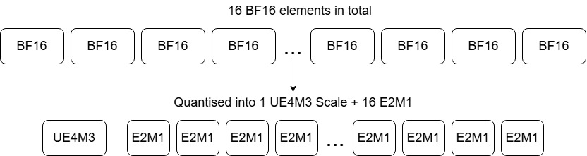
What’s a scale and what’s a block? Although the name NVFP4 suggests 4-bit, the storage itself really is 4.5-bit per element. A BF16 number is 16 bits. An NVFP4 tensor stores each element as a 4-bit E2M1 code and adds one 8-bit scale for every block of 16 elements, so the cost per element is
$$ \frac{16 \times 4 + 8}{16} = 4.5 \text{ bits} \tag{5} $$For E2M1, its representable values are just 15 levels:
$$ x \in \{0,\ \pm 0.5,\ \pm 1,\ \pm 1.5,\ \pm 2,\ \pm 3,\ \pm 4,\ \pm 6\} \tag{6} $$If we quantise every value in the query by mapping it to one of these 15 levels, accuracy will drop significantly. This is because, for example, mapping the highest value 1000 to 6.0, while a big chunk of the values are in the range 10-15, will cause all these values to be mapped into a single level (0) within the 15 levels, even though they differ in magnitude within the range of 10-15, causing the total error to spike. Thus, this brings out our first concept – block. Instead of quantising per query tensor, we quantise per block (16 BF16 elements), so the min-max range can be a smaller difference in magnitude, preserving the error rate.
However, blocks are not enough, we also need a scale that differs by block because the magnitude of each block’s elements differs. By dividing by the scale, we can further reduce the min and max range to [-6, 6], significantly reducing potential quantisation error. An example of the calculation can be shown here:
$$ x = [\,3.1,\ -1.2,\ 0.4,\ 5.9,\ 2.2,\ -0.7,\ 1.6,\ 4.4\,],\qquad \max|x_i| = 5.9 $$$$ s = 5.9/6 \approx 1.0 $$$$ \hat{x} = \text{round to nearest E2M1 value}(x/s) $$$$ \hat{x} = [\,3,\ -1,\ 0.5,\ 6,\ 2,\ -0.5,\ 1.5,\ 4\,],\qquad \\ error = [\,-0.1,\ 0.2,\ 0.1,\ 0.1,\ -0.2,\ 0.2,\ -0.1,\ \mathbf{-0.4}\,] $$Every element has relatively small quantisation error except for the last one that falls into the wide 4->6 gap, this is the exact motivation for fouroversix.
FourOverSix
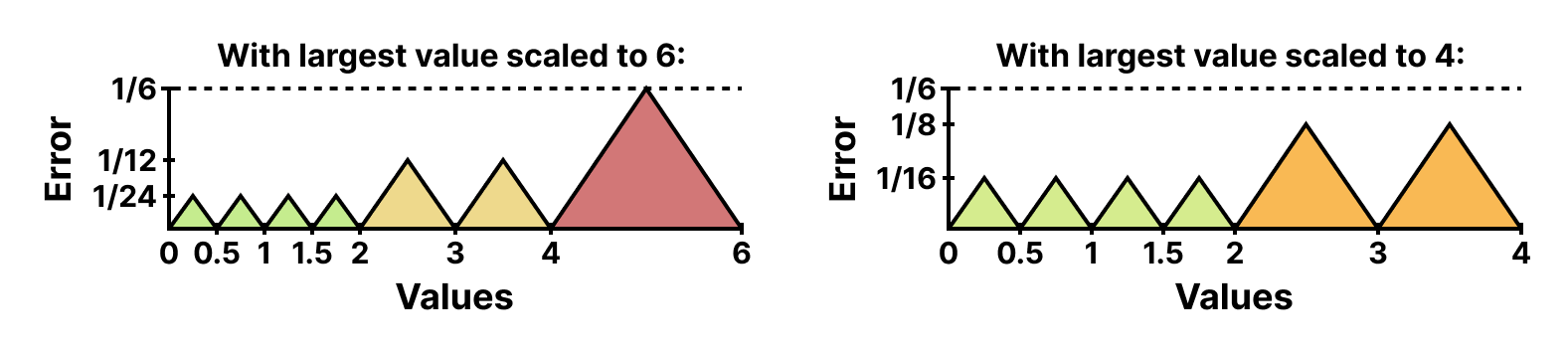 Image extracted from [4]
The main idea in fouroversix is that “max on 6” isn’t always best for quantisation; it depends on the range of the values. amax/4 beats amax/6 when a block has multiple elements clustered near its own maximum. If we use amax/6 on these data, the multiple elements clustered near the max will fall into the 4->6 gap, magnifying the quantisation error. Hence the idea here is to use amax/4 or amax/6 dynamically. When a block has multiple elements clustered near the maximum, use amax/4, and if a block has a more evenly spread distribution, use amax/6. You might be wondering how a kernel determines which amax to use in real time. Basically, we compute the Mean Squared Error for each amax and then calculate the score. It doubles the amount of work, but accuracy is recovered, so it’s a trade-off.
Let’s visualise the amax/4 example using the same data:
$$ s' = (5.9/4) \approx 1.5\qquad \hat{x}' = [\,2,\ -1,\ 0.5,\ 4,\ 1.5,\ -0.5,\ 1,\ 3\,] $$$$ error = [\,-0.1,\ -0.3,\ 0.35,\ 0.1,\ 0.05,\ -0.05,\ -0.1,\ 0.1\,] $$The large values are now much better, though at the expense of the small ones. Neither divisor is always right, so the quantiser has to try every time and keep the one with the smallest squared error.
2. CuteDSL Kernel
The computation of the Q and K
As mentioned above, self-attention is our primary target for implementing NVFP4 acceleration because DiT spends most of its time in self-attention due to the large intermediate state they need to compute. Recall that, for each attention head (24 attention heads in total, and each head dimension is 128), we need to multiply the query (7040 tokens) by the keys (28160 tokens).
$$ S = \frac{Q K^{\top}}{\sqrt{d}} \in \mathbb{R}^{7040 \times 28160},\qquad Q \in \mathbb{R}^{7040 \times 128},\ K \in \mathbb{R}^{28160 \times 128} \tag{7} $$$$ 7040 \times 28160 \times 4\ \text{B} = 793\ \text{MB per head} \tag{8} $$We never materialise the full 7040 x 28160 due to TMEM and SMEM limitations, instead, we divide them into 128-token pages. And even if we materialise them, the GPU would spend most of its time reading the data instead of computing the data, because now we can’t overlap compute and memory load. Hence, it’s really 7040/128=55 tiles of queries, together with 220 pages of keys. Precisely, we cut $Q$ into 128-row tiles and $K$ into 128-key pages, and one MMA handles one (tile, page) pair:
$$ S^{(t,p)} = Q^{(t)} \big(K^{(p)}\big)^{\top} \in \mathbb{R}^{128 \times 128},\qquad t = 1..\tfrac{7040}{128} = 55,\quad p = 1..\tfrac{28160}{128} = 220 \tag{9} $$so a head is $55 \times 220 = 12{,}100$ such tiles, and a call over 24 heads is $290{,}400$.
When does dequantisation happen?
You must be wondering where the dequantisation happens. Note that the tensor core never really rebuilds the dequantised tensor independently, instead, it fuses it with the block-scaled MMA instruction, which multiplies the q and k and applies the two scales per 16-element chunk inside the dot product:
$$ \sum_{i=1}^{128} q_i\, k_i \;\approx\; \sum_{g=1}^{8} s^{q}_{g}\, s^{k}_{g} \sum_{i = 16(g-1)+1}^{16g} \hat{q}_i\, \hat{k}_i \tag{10} $$Online Softmax
And of course, we can always merge the multiplication of $O=PV$ values into the same kernel to output the ultimate state. Note that softmax has to be applied along each query row, over all 28160 keys, involving every element, because $P=softmax(S)$, even if we are not materialising the full intermediate state. In this case, we use online softmax [5]. The main problem online softmax tries to solve is that, given we only materialise a 128x128 tile at a time, we want to compute the row max and sum while computing the softmax, without another pass. In mathematical terms, when we are computing the softmax, the equation is:
$$ P_k = \frac{e^{S_k}}{\sum_{j=1}^{28160} e^{S_j}}, \quad k = 1 … 28160 $$Furthermore, in FP32, the $e^{S}$ will blow up if $S>88$, hence we also need to calculate $e^{S-m}$, where $m$ is the current max of $S_k$, instead of $e^{S}$.
$$ P_k = \frac{e^{S_k - m}}{\sum_{j=1}^{28160} e^{S_j - m}}, \quad k = 1 … 28160 $$Based on this information, we need to track both the max and the sum at the same time.
In online softmax, we need to keep 3 things:
- $m$, the running max for the logits seen so far
- $\ell$ running sum $\sum {e^{S_k - m}}$ over all the keys seen so far, relative to the current $m$.
- $o$ running output $\sum {e^{S_k - m}} V_k$, likewise over all the keys seen so far, relative to the current $m$.
The above three variables are instrumental in supporting online softmax, because the main trick of it is to carry a provisional max and running sum, and then fix it up later. The main idea is that even if we have found a new max in a new 128x128 tile, it is very easy to update the above three variables to the correct values by just one multiplication, because:
$$ \sum_{k \in \text{old}} e^{S_k - m_{\text{new}}} = e^{m_{\text{old}} - m_{\text{new}}} \sum_{k \in \text{old}} e^{S_k - m_{\text{old}}} $$Hence, for every key in each tile, the updates that need to be done are:
$$ m_{\text{new}} = max(m, S_k) \\ \alpha = e^{m-m_{\text{new}}} \\ \ell = \alpha \ell + e^{S_k - m_{\text{new}}} \\ o = \alpha o + e^{S_k - m_{\text{new}}} V_k \\ m = m_{\text{new}} \\ $$and finally,
$$ o_{final} = \frac{o_{\text{last tile}}}{\ell_{\text{last tile}}} $$Where do the tiles live?
 Image extracted from [6]
After understanding the types of computation involved in the kernel, let’s work on understanding how the tiles live and move from a CuteDSL perspective. The famous problem in the MLSys world is the “memory wall” problem. When the compute engine is computing much faster than the speed of fetching data, we need to speed up the data transfer to avoid the GPU being idle. When data transfer hits a bandwidth limit due to physical constraints, we introduce a memory hierarchy to provide cache locality for recently used data. We also pipeline compute and data movement to overlap them, hoping to extract every possible performance gain.
In a GPU context, the data we need for self-attention, namely Q, K and V tiles, first live in the Global Memory (GMEM) because they can’t all fit into the GPU cache. As the kernel computes tile by tile, the data will be moved from the GMEM to Shared Memory (SMEM), and then directly used by Tensor Cores, units nearest to the compute cores, so that the matmul can happen, before the intermediate output is accumulated into Tensor Memory (TMEM, first introduced in Blackwell), and then the fully computed answer is sent to Register Memory (RMEM) and finally back to SMEM and GMEM.
To break down all the memory operations for this specific kernel, I have prepared this table as a summary:
| Direction | Code |
|---|---|
| GMEM -> SMEM (Q, K, V pages and their scales) | cpasync.CopyBulkTensorTileG2SOp (TMA) |
| SMEM -> TMEM (block scales only: SFQ, SFK, SFV, SFP) | tcgen05.make_s2t_copy |
| SMEM + TMEM -> tensor core -> TMEM, MMA #1 | cute.gemm(…), completion via tcgen05.commit(mbarrier), and tcgen05.mma.kind::mxf4nvf4.block_scale |
| TMEM + SMEM -> tensor core -> TMEM, MMA #2 (A = P from TMEM, B = V from SMEM) | tcgen05.mma.kind::mxf4nvf4.block_scale |
| TMEM -> RMEM (S out to the softmax warps) | tcgen05.Ld32x32bOp |
| RMEM (online softmax + P quantisation) | ex2.approx, rcp.approx, cvt.rn.satfinite.e2m1x2 |
| RMEM -> TMEM (P back as the A operand of MMA #2) | tcgen05.st |
| RMEM -> SMEM (SFP scales, correction factors) | st.shared + fence.proxy.async |
| TMEM -> RMEM -> TMEM (correction: rescale O when the running max moved) | tcgen05.ld -> multiply -> tcgen05.st |
| TMEM -> RMEM -> SMEM -> GMEM (epilogue, after the last page) | tcgen05.ld -> rcp.approx(ℓ) -> st.shared -> cpasync.CopyBulkTensorTileS2GOp (TMA store) |
| Synchronisation (every hand-off above) | tcgen05.fence, mbarrier, cute.arch.mbarrier_init_fence(), cute.arch.barrier() |
| TMEM lifecycle (once per CTA) | tcgen05.alloc / tcgen05.dealloc |
Summary
That’s about it for now. From here, we have seen how NVIDIA has created multiple tiers of memory hierarchy to hide the memory wall problem. On a random note, we have observed that the computational bottleneck has shifted from GEMM to softmax instead, which signifies that the next generation of architecture might have to target this portion of the transformer code or else the tensor core would be idle most of the time as well, no matter how fast it is now.
Reference
- Xiao, Guangxuan, et al. “Efficient streaming language models with attention sinks.” International Conference on Learning Representations. Vol. 2024. 2024.
- Yang, Shuai, et al. “Longlive: Real-time interactive long video generation.” arXiv preprint arXiv:2509.22622 (2025).
- Peebles, William, and Saining Xie. “Scalable diffusion models with transformers.” 2023 IEEE/CVF International Conference on Computer Vision (ICCV). IEEE, 2023.
- Cook, Jack, et al. “Four over six: More accurate nvfp4 quantization with adaptive block scaling.” arXiv preprint arXiv:2512.02010 (2025).
- Milakov, Maxim, and Natalia Gimelshein. “Online normalizer calculation for softmax.” arXiv preprint arXiv:1805.02867 (2018).
- Modern GPU Programming for MLSys. MLC Community, 2026, mlc.ai/modern-gpu-programming-for-mlsys/index.html. Accessed 25 Sept. 2026.